![]()
![]()
The goal of splinetrials is to analyze longitudinal clinical data applying natural cubic splines to a continuous time variable.
Install this package from CRAN with:
install.packages("splinetrials")You can also install the development version of splinetrials from GitHub with:
# install.packages("pak")
pak::pak("NikKrieger/splinetrials")library(survival)
library(mmrm)
library(splinetrials)
library(dplyr)
#>
#> Attaching package: 'dplyr'
#> The following objects are masked from 'package:stats':
#>
#> filter, lag
#> The following objects are masked from 'package:base':
#>
#> intersect, setdiff, setequal, union
library(ggplot2)The NCS model is a longitudinal mixed model of repeated measures (MMRM) with random effects marginalized out, additive baseline covariates, and time parameterized using natural cubic splines.
The package functions accept data sets with one row per patient per scheduled visit (including baseline).
We’ll adapt the pbcseq data set in the survival
package:
pbcseq_mod <-
  survival::pbcseq |>
  mutate(
    years = day / 365.25,
    visit_index =
      bin_timepoints( # splinetrials helper function yielding an ordered factor
        observed = years,
        scheduled = c(0, 0.5, 1:round(max(years))),
        labels = c("Baseline", paste(c(0.5, 1:round(max(years))), "yr"))
      ),
    sch_visit_years = c(0, 0.5, 1:round(max(years)))[as.numeric(visit_index)],
    sch_visit_label = as.character(visit_index),
    trt = factor(trt, labels = c("control", "treatment"))
  ) |>
  arrange(id, visit_index, abs(years - sch_visit_years)) |>
  distinct(id, visit_index, .keep_all = TRUE) |>
  select(id, visit_index:sch_visit_label, trt, everything()) |>
  as_tibble()

pbcseq_mod
#> # A tibble: 1,906 × 23
#>       id visit_index sch_visit_years sch_visit_label trt     futime status   age
#>    <int> <ord>                 <dbl> <chr>           <fct>    <int>  <int> <dbl>
#>  1     1 Baseline                0   Baseline        treatm…    400      2  58.8
#>  2     1 0.5 yr                  0.5 0.5 yr          treatm…    400      2  58.8
#>  3     2 Baseline                0   Baseline        treatm…   5169      0  56.4
#>  4     2 0.5 yr                  0.5 0.5 yr          treatm…   5169      0  56.4
#>  5     2 1 yr                    1   1 yr            treatm…   5169      0  56.4
#>  6     2 2 yr                    2   2 yr            treatm…   5169      0  56.4
#>  7     2 5 yr                    5   5 yr            treatm…   5169      0  56.4
#>  8     2 6 yr                    6   6 yr            treatm…   5169      0  56.4
#>  9     2 7 yr                    7   7 yr            treatm…   5169      0  56.4
#> 10     2 8 yr                    8   8 yr            treatm…   5169      0  56.4
#> # ℹ 1,896 more rows
#> # ℹ 15 more variables: sex <fct>, day <int>, ascites <int>, hepato <int>,
#> #   spiders <int>, edema <dbl>, bili <dbl>, chol <int>, albumin <dbl>,
#> #   alk.phos <int>, ast <dbl>, platelet <int>, protime <dbl>, stage <int>,
#> #   years <dbl>
Notice how the helper function
splinetrials::bin_timepoints() creates the visit index,
categorizing follow-up visits based on when they were scheduled (see
?survival::pbcseq).
Once we have these variables created, we are ready for a full NCS
analysis using ncs_analysis(). This produces a table of
summary statistics, including LS means and confidence intervals:
pbc_spline_analysis <-
  ncs_analysis(
    data = pbcseq_mod,
    response = alk.phos,
    subject = id,
    arm = trt,
    control_group = "control",
    time_observed_continuous = years,
    time_observed_index = visit_index,
    time_scheduled_continuous = sch_visit_years,
    time_scheduled_label = sch_visit_label,
    covariates = ~ age + sex + bili + albumin + ast + protime
  )
#> → The covariance structure `"us"` did not successfully converge.
#> Warning in mmrm::mmrm(method = "Satterthwaite", formula = alk.phos ~
#> spline_fn(years)[, : Divergence with optimizer L-BFGS-B due to problems:
#> L-BFGS-B needs finite values of 'fn'
#> mmrm() registered as emmeans extension
pbc_spline_analysis
#> # A tibble: 32 × 32
#>    arm     time         n   est    sd    se lower upper response_est response_se
#>    <fct>   <chr>    <int> <dbl> <dbl> <dbl> <dbl> <dbl>        <dbl>       <dbl>
#>  1 control Baseline   154 1943. 2102. 169.  1611. 2275.        1424.        77.0
#>  2 control 0.5 yr     131 1574. 1134.  99.1 1379. 1768.        1377.        71.9
#>  3 control 1 yr       130 1543.  934.  81.9 1382. 1703.        1330.        68.6
#>  4 control 2 yr       111 1481. 1076. 102.  1281. 1681.        1243.        67.2
#>  5 control 3 yr        83 1252.  662.  72.7 1110. 1395.        1169.        69.1
#>  6 control 4 yr        75 1182.  716.  82.7 1020. 1344.        1107.        71.0
#>  7 control 5 yr        61 1250.  902. 115.  1023. 1476.        1058.        71.1
#>  8 control 6 yr        56 1073.  589.  78.7  919. 1228.        1019.        69.4
#>  9 control 7 yr        47 1022.  601.  87.6  851. 1194.         989.        66.6
#> 10 control 8 yr        37 1021.  554.  91.1  842. 1199.         968.        64.4
#> # ℹ 22 more rows
#> # ℹ 22 more variables: response_df <dbl>, response_lower <dbl>,
#> #   response_upper <dbl>, change_est <dbl>, change_se <dbl>, change_df <dbl>,
#> #   change_lower <dbl>, change_upper <dbl>, change_test_statistic <dbl>,
#> #   change_p_value <dbl>, diff_est <dbl>, diff_se <dbl>, diff_df <dbl>,
#> #   diff_lower <dbl>, diff_upper <dbl>, diff_test_statistic <dbl>,
#> #   diff_p_value <dbl>, percent_slowing_est <dbl>, …
Note that the above warnings are expected, as splinetrials and
mmrm::mmrm() iterate through different covariance
structures and optimizers until a converging model is achieved.
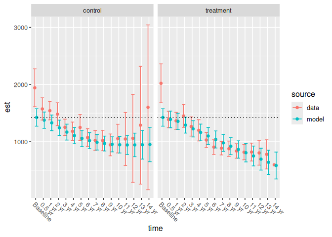
We can plot the resulting model against the data by feeding the
resulting data set to ncs_plot_means():
p1 <- ncs_plot_means(pbc_spline_analysis)
p1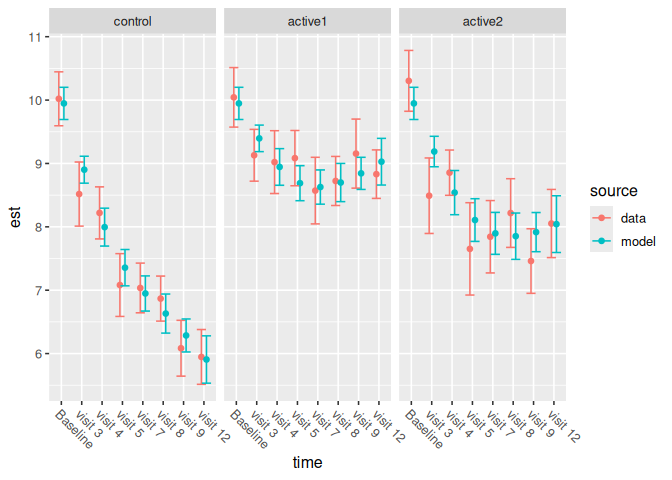
The parameterization has additive effects and pairwise interactions for study arm and time point (i.e., spline basis functions). The model is constrained so that all study arms have equal means at baseline: notice that the same line passes through both the control group’s and the treatment group’s modeled mean baseline estimates:
p1 +
  geom_hline(
    aes(yintercept = response_est),
    data = filter(pbc_spline_analysis, time == "Baseline"),
    linetype = 3
  )
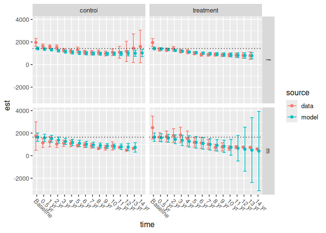
Run a NCS analysis with subgroups using
ncs_analysis_subgroup(). The data set should include a
categorical variable to indicate subgroup membership. In this case, the
sex variable serves as the subgroup.
subgroup_analysis_results <-
  ncs_analysis_subgroup(
    data = pbcseq_mod,
    response = alk.phos,
    subject = id,
    arm = trt,
    control_group = "control",
    subgroup = sex,
    subgroup_comparator = "f",
    time_observed_continuous = years,
    time_observed_index = visit_index,
    time_scheduled_continuous = sch_visit_years,
    time_scheduled_label = sch_visit_label,
    covariates = ~ age + bili + albumin + ast + protime,
    cov_structs = "ar1h",
    return_models = TRUE
  )
#> mmrm() registered as car::Anova extension
#> Warning in mmrm::mmrm(formula = alk.phos ~ spline_fn(years)[, 1] +
#> spline_fn(years)[, : Divergence with optimizer L-BFGS-B due to problems:
#> L-BFGS-B needs finite values of 'fn'
#> Warning in mmrm::mmrm(formula = alk.phos ~ spline_fn(years)[, 1] +
#> spline_fn(years)[, : Divergence with optimizer L-BFGS-B due to problems:
#> L-BFGS-B needs finite values of 'fn'
This function returns a list of multiple analyses, which are better looked at one at a time:
The between and within tables contain the
same data except for the treatment effect columns. Note also that they
are sorted differently.
betweenThe between table calculates treatment effects between
the subgroups within each study arm:
subgroup_analysis_results$between
#> # A tibble: 62 × 30
#>    arm       time     subgroup     n   est    sd    se lower upper response_est
#>    <fct>     <chr>    <fct>    <int> <dbl> <dbl> <dbl> <dbl> <dbl>        <dbl>
#>  1 control   Baseline f          139 1966. 2066. 175.  1622. 2309.        1429.
#>  2 control   Baseline m           15 1734. 2478. 640.   480. 2989.        1640.
#>  3 treatment Baseline f          137 1950. 2151. 184.  1590. 2310.        1429.
#>  4 treatment Baseline m           21 2486. 2385. 521.  1466. 3506.        1640.
#>  5 control   0.5 yr   f          119 1619. 1162. 106.  1410. 1827.        1377.
#>  6 control   0.5 yr   m           12 1134.  714. 206.   730. 1538.        1572.
#>  7 treatment 0.5 yr   f          108 1348.  818.  78.7 1194. 1502.        1385.
#>  8 treatment 0.5 yr   m           17 1646.  821. 199.  1256. 2037.        1592.
#>  9 control   1 yr     f          118 1575.  944.  86.9 1405. 1745.        1325.
#> 10 control   1 yr     m           12 1229.  796. 230.   778. 1679.        1506.
#> # ℹ 52 more rows
#> # ℹ 20 more variables: response_se <dbl>, response_df <dbl>,
#> #   response_lower <dbl>, response_upper <dbl>, change_est <dbl>,
#> #   change_se <dbl>, change_df <dbl>, change_lower <dbl>, change_upper <dbl>,
#> #   change_test_statistic <dbl>, change_p_value <dbl>, diff_subgroup_est <dbl>,
#> #   diff_subgroup_se <dbl>, diff_subgroup_df <dbl>, diff_subgroup_lower <dbl>,
#> # diff_subgroup_upper <dbl>, diff_subgroup_test_statistic <dbl>, …withinThe within table calculates treatment effects between
each study arm within each subgroup:
subgroup_analysis_results$within
#> # A tibble: 62 × 33
#>    arm     time     subgroup     n   est    sd    se lower upper response_est
#>    <fct>   <chr>    <fct>    <int> <dbl> <dbl> <dbl> <dbl> <dbl>        <dbl>
#>  1 control Baseline f          139 1966. 2066. 175.  1622. 2309.        1429.
#>  2 control 0.5 yr   f          119 1619. 1162. 106.  1410. 1827.        1377.
#>  3 control 1 yr     f          118 1575.  944.  86.9 1405. 1745.        1325.
#>  4 control 2 yr     f          100 1527. 1109. 111.  1310. 1744.        1230.
#>  5 control 3 yr     f           74 1271.  685.  79.6 1115. 1427.        1151.
#>  6 control 4 yr     f           68 1193.  743.  90.2 1016. 1369.        1088.
#>  7 control 5 yr     f           54 1297.  949. 129.  1044. 1550.        1040.
#>  8 control 6 yr     f           49 1093.  619.  88.5  920. 1266.        1005.
#>  9 control 7 yr     f           40 1049.  641. 101.   850. 1247.         981.
#> 10 control 8 yr     f           31 1088.  575. 103.   885. 1290.         969.
#> # ℹ 52 more rows
#> # ℹ 23 more variables: response_se <dbl>, response_df <dbl>,
#> #   response_lower <dbl>, response_upper <dbl>, change_est <dbl>,
#> #   change_se <dbl>, change_df <dbl>, change_lower <dbl>, change_upper <dbl>,
#> #   change_test_statistic <dbl>, change_p_value <dbl>, diff_arm_est <dbl>,
#> #   diff_arm_se <dbl>, diff_arm_df <dbl>, diff_arm_lower <dbl>,
#> # diff_arm_upper <dbl>, diff_arm_test_statistic <dbl>, …We can supply either of the above result entries (i.e.,
between or within) to
ncs_plot_means_subgroup(). This function creates a grid of
plots that again depict the actual and modeled mean responses at each
timepoint. Each column of plots contains a study arm and each row of
plots contains a subgroup.
We again include horizontal lines to demonstrate that the study arms all have the same modeled mean baseline estimate:
ncs_plot_means_subgroup(subgroup_analysis_results$between) +
  geom_hline(
    aes(yintercept = response_est),
    data = filter(subgroup_analysis_results$between, time == "Baseline"),
    linetype = 3,
    lwd = 0.5
  )
type3 contains a Type-III ANOVA on the main analysis
model’s terms:
subgroup_analysis_results$type3
#> # A tibble: 14 × 6
#> effect chisquare_test_stati…¹ df p_value correlation optimizer
#> <chr> <dbl> <int> <dbl> <chr> <chr>
#> 1 spline_fn(years)[… 30.2 1 3.84e-8 heterogene… mmrm+tmb
#> 2 spline_fn(years)[… 13.5 1 2.43e-4 heterogene… mmrm+tmb
#> 3 sex 1.26 1 2.62e-1 heterogene… mmrm+tmb
#> 4 age 23.5 1 1.24e-6 heterogene… mmrm+tmb
#> 5 bili 6.08 1 1.37e-2 heterogene… mmrm+tmb
#> 6 albumin 7.16 1 7.45e-3 heterogene… mmrm+tmb
#> 7 ast 2.95 1 8.57e-2 heterogene… mmrm+tmb
#> 8 protime 1.76 1 1.85e-1 heterogene… mmrm+tmb
#> 9 spline_fn(years)[… 1.20 1 2.74e-1 heterogene… mmrm+tmb
#> 10 spline_fn(years)[… 2.70 1 1.01e-1 heterogene… mmrm+tmb
#> 11 spline_fn(years)[… 0.000212 1 9.88e-1 heterogene… mmrm+tmb
#> 12 spline_fn(years)[… 1.29 1 2.56e-1 heterogene… mmrm+tmb
#> 13 spline_fn(years)[… 0.0588 1 8.08e-1 heterogene… mmrm+tmb
#> 14 spline_fn(years)[… 0.0164 1 8.98e-1 heterogene… mmrm+tmb
#> # ℹ abbreviated name: ¹chisquare_test_statisticThe optional interaction result contains an ANOVA
comparing the original model fit to a reduced version:
subgroup_analysis_results$interaction
#>           model      aic      bic    loglik -2*log(l) test_statistic df
#> 1 reduced model 29201.78 29314.07 -14570.89  29141.78             NA NA
#> 2    full model 29205.64 29325.42 -14570.82  29141.64      0.1351363  2
#>    p_value                          correlation optimizer
#> 1       NA heterogeneous autoregressive order 1  mmrm+tmb
#> 2 0.934664 heterogeneous autoregressive order 1  mmrm+tmb
return_models = TRUELastly, the user can optionally obtain the original analysis model
object as well as those used for the subgroup interaction test, which
are returned as the analysis_model, full, and
reduced entries. These are mmrm objects
created using mmrm::mmrm(). Here is
analysis_model, for example:
subgroup_analysis_results$analysis_model
#> mmrm fit
#>
#> Formula:     alk.phos ~ spline_fn(years)[, 1] + spline_fn(years)[, 2] + sex +
#>     age + bili + albumin + ast + protime + spline_fn(years)[,
#>     1]:sex + spline_fn(years)[, 2]:sex + spline_fn(years)[, 1]:trt +
#>     spline_fn(years)[, 2]:trt + spline_fn(years)[, 1]:sex:trt +
#>     spline_fn(years)[, 2]:sex:trt
#> Data:        dplyr::mutate(pbcseq_mod, sex = factor(sex, c("f", "m"))) (used
#> 1860 observations from 312 subjects with maximum 16 timepoints)
#> Covariance:  heterogeneous auto-regressive order one (17 variance parameters)
#> Inference:   REML
#> Deviance:    29002.11
#>
#> Coefficients:
#>                             (Intercept)                   spline_fn(years)[, 1]
#>                             2721.322358                             -815.000265
#>                   spline_fn(years)[, 2]                                    sexm
#>                             -217.027228                              210.533944
#>                                     age                                    bili
#>                              -18.112882                               22.507712
#>                                 albumin                                     ast
#>                              -95.578177                                1.296681
#>                                 protime              spline_fn(years)[, 1]:sexm
#>                              -28.763036                             -458.009692
#>              spline_fn(years)[, 2]:sexm      spline_fn(years)[, 1]:trttreatment
#>                             -478.555152                              -53.251556
#>      spline_fn(years)[, 2]:trttreatment spline_fn(years)[, 1]:sexm:trttreatment
#>                             -299.228629                              113.096456
#> spline_fn(years)[, 2]:sexm:trttreatment
#>                              -78.148527
#>
#> Model Inference Optimization:
#> Converged with code 0 and message: convergence: rel_reduction_of_f <= factr*epsmchThe basic NCS analysis results table pbc_spline_analysis
has one row per study arm per timepoint of interest and the following
columns:
arm: study arm, i.e. treatment grouptime: discrete visit time labels from the
time_scheduled_label column in the data.n: number of non-missing observations.est: observed mean response in the data.sd: observed standard deviation of the response in the
data.se: observed standard error of the response in the data
(just se / sqrt(n)).lower: lower bound of an observed 95% confidence
interval in the data.upper: upper bound of an observed 95% confidence
interval in the data.response_est: LS mean of the response.response_se: standard error of the LS mean of the
response.response_df: degrees of freedom of the LS mean of the
response.response_lower: lower 95% confidence bound of the LS
mean of the response.response_upper: upper 95% confidence bound of the LS
mean of the response.change_est, change_lower,
change_upper, change_se,
change_df: like the analogous response_*
columns, but for LS mean change from baseline.change_test_statistic: test statistic of a two-sided
test that the LS mean change from baseline is not equal to 0, at a
significance level of 5%.change_p_value: same as
change_test_statistic, but the p-value instead of the test
statistic.diff_est, diff_se, diff_df,
diff_lower, diff_upper,
diff_test_statistic, diff_p_value: same as the
analogous change_* columns, but for treatment
differences.percent_slowing_est LS mean of percent slowing (on the
percentage scale).percent_slowing_lower,
percent_slowing_upper: a conservative approximation to a
confidence interval on percent slowing. Assumes uncorrelated changes
from baseline.correlation: correlation structure of the whole
model.optimizer: optimization algorithm for the whole
model.between and
within tablesThe between-subgroup and within-subgroup tables have one row per study arm per timepoint per subgroup and the following columns:
arm: study arm, i.e. treatment grouptime: discrete visit time labels from the
time_scheduled_label column in the data.subgroup: subgroup leveln: number of non-missing observations.est: observed mean response in the data.sd: observed standard deviation of the response in the
data.se: observed standard error of the response in the data
(just se / sqrt(n)).lower: lower bound of an observed 95% confidence
interval in the data.upper: upper bound of an observed 95% confidence
interval in the data.response_est: LS mean of the response.response_se: standard error of the LS mean of the
response.response_df: degrees of freedom of the LS mean of the
response.response_lower: lower 95% confidence bound of the LS
mean of the response.response_upper: upper 95% confidence bound of the LS
mean of the response.change_est, change_lower,
change_upper, change_se,
change_df: like the analogous response_*
columns, but for LS mean change from baseline.change_test_statistic: test statistic of a two-sided
test that the LS mean change from baseline is not equal to 0, at a
significance level of 5%.change_p_value: same as
change_test_statistic, but the p-value instead of the test
statistic.diff_arm_est, diff_arm_se,
diff_arm_df, diff_arm_lower,
diff_arm_upper, diff_arm_test_statistic,
diff_arm_p_value: same as the analogous
change_* columns, but for treatment differences.diff_subgroup_est, diff_subgroup_se,
diff_subgroup_df, diff_subgroup_lower,
diff_subgroup_upper,
diff_subgroup_test_statistic,
diff_subgroup_p_value: same as the analogous
*_arm_* columns, but for the subgroup differences.percent_slowing_est LS mean of percent slowing (on the
percentage scale).percent_slowing_lower,
percent_slowing_upper: a conservative approximation to a
confidence interval on percent slowing. Assumes uncorrelated changes
from baseline.correlation: correlation structure of the analysis
subgroup model.optimizer: optimizer of the analysis subgroup
model.type3 column
descriptionsThe Type-III ANOVA table has one row per effect in the main analysis model and the following columns:
effect: the model effect in the main analysis
modelchisquare_test_statistic: Chi-squared test statistic
for the model term’s significancedf: degrees of freedomp_value: p-value for the test of the model term’s
significancecorrelation: correlation structure of the analysis
subgroup model.optimizer: optimizer of the analysis subgroup
model.interaction column
descriptionsThe subgroup interaction test table will have two rows: the first will represent the reduced model and the second will depict the full model. Likelihood ratio test results will only be in the latter row. The table will contain the following columns:
model: the model, either full or reduced.df: degrees of freedomaic: Akaike Information Criterionbic: Bayesian Information Criterionloglik: log likelihoodtest_statistic: test statistic of the likelihood ratio
test.p_value: p-value of the likelihood ratio test.correlation: correlation structures of the full and
reduced models of the interaction test.optimizer: optimizers of the full and reduced models of
the interaction test.