![]()
![]()
Supervised Variational Autoencoder (VAE) regression for high‑dimensional predictors (e.g., VIS–NIR–SWIR soil spectroscopy), implemented in Python TensorFlow/Keras and exposed in R via reticulate.
The README is also the main reproducible case study,
mirroring the vignette (vignettes/soilVAE-workflow.Rmd) so
a reader can understand the why, how, and
performance without opening additional files.
Given spectra \(x\in\mathbb{R}^p\) and a continuous soil property \(y\in\mathbb{R}\), soilVAE learns:
We minimize a weighted sum:
\[ \mathcal{L}(x,y) = \underbrace{\|x-\hat x\|_2^2}_{\text{reconstruction}} \;+\; \beta\;\underbrace{D_{KL}\!\left(q_\phi(z\mid x)\,\|\,\mathcal{N}(0,I)\right)}_{\text{regularization}} \;+\; \alpha\;\underbrace{\|y-\hat y\|_2^2}_{\text{regression}}. \]
In the package API, these correspond to beta_kl = β and
alpha_y = α.
install.packages("soilVAE")# install.packages("remotes")
remotes::install_github("HugoMachadoRodrigues/soilVAE")Because deep learning depends on external Python libraries, this README uses a defensive pattern:
Important:
reticulate“locks” the Python used per R session. If you change env variables oruse_*()calls, restart R.
library(reticulate)

# Make sure reticulate isn't forced to a missing python
Sys.unsetenv("RETICULATE_PYTHON")

# Create env (if needed)
if (!"soilvae-tf" %in% conda_list()$name) {
  conda_create("soilvae-tf", python_version = "3.11")
}

# Install core deps from conda-forge
conda_install("soilvae-tf", packages = c("pip", "numpy"), channel = "conda-forge")

# Install TF/Keras via pip inside the env
py_install(c("tensorflow>=2.13", "keras>=3"), pip = TRUE, envname = "soilvae-tf")
Now, in the same R session:
library(soilVAE)
soilVAE::vae_configure(conda = "soilvae-tf")
reticulate::py_config()library(soilVAE)
soilVAE::vae_configure(python = "C:/path/to/python.exe")This follows the workflow style commonly used in soil spectral inference tutorials (e.g., Wadoux et al., 2021) (Wadoux et al. 2021), with a direct comparison between a PLS baseline and soilVAE.
set.seed(19101991)

pkgs <- c("prospectr", "pls", "reticulate")
for (p in pkgs) if (!requireNamespace(p, quietly = TRUE)) install.packages(p)

library(prospectr)
library(pls)
library(reticulate)

if (!requireNamespace("soilVAE", quietly = TRUE)) {
  stop("soilVAE is not installed. Install it with remotes::install_github('HugoMachadoRodrigues/soilVAE').")
}
library(soilVAE)

# Defensive: detect Python + TF/Keras early, so the README can render everywhere.
has_py <- reticulate::py_available(initialize = FALSE)
has_tf <- FALSE
if (has_py) {
  try(reticulate::py_config(), silent = TRUE)
  has_tf <- reticulate::py_module_available("tensorflow") &&
    reticulate::py_module_available("keras")
}This example assumes you ship datsoilspc inside the
package (data/datsoilspc.rda).
This dataset is provided and described at Geeves et al. (1995)
Geeves, G. W. (Guy W.) & New South Wales. Department of Conservation and Land Management & CSIRO. Division of Soils. (1995). The physical, chemical and morphological properties of soils in the wheat-belt of southern N.S.W. and northern Victoria / G.W. Geeves … [et al.]. Glen Osmond, S. Aust. : CSIRO Division of Soils
data("datsoilspc", package = "soilVAE")
str(datsoilspc)
#> 'data.frame':    391 obs. of  5 variables:
#>  $ clay       : num  49 7 56 14 53 24 9 18 33 27 ...
#>  $ silt       : num  10 24 17 19 7 21 9 20 13 19 ...
#>  $ sand       : num  42 69 27 67 40 55 83 61 54 55 ...
#>  $ TotalCarbon: num  0.15 0.12 0.17 1.06 0.69 2.76 0.66 1.36 0.19 0.16 ...
#>  $ spc        : num [1:391, 1:2151] 0.0898 0.1677 0.0778 0.0958 0.0359 ...
#>   ..- attr(*, "dimnames")=List of 2
#>   .. ..$ : NULL
#>   .. ..$ : chr [1:2151] "350" "351" "352" "353" ...
#>  - attr(*, "na.action")= 'omit' Named int 392
#>   ..- attr(*, "names")= chr "63"
Expected structure:
datsoilspc$spc: matrix of reflectance spectra (rows =
samples; cols = wavelengths)datsoilspc$TotalCarbon: numeric target (example
property)We replicate typical “quantitative” metrics used in soil
spectroscopy:
RMSE, MAE, R², bias (ME), RPIQ, and RPD.
eval_quant <- function(y, yhat) {
  y <- as.numeric(y)
  yhat <- as.numeric(yhat)

  ok <- is.finite(y) & is.finite(yhat)
  y <- y[ok]
  yhat <- yhat[ok]

  if (length(y) < 3) {
    return(list(
      n = length(y),
      ME = NA_real_, MAE = NA_real_, RMSE = NA_real_,
      R2 = NA_real_, RPIQ = NA_real_, RPD = NA_real_
    ))
  }

  err <- yhat - y
  me <- mean(err)
  mae <- mean(abs(err))
  rmse <- sqrt(mean(err^2))

  ss_res <- sum((y - yhat)^2)
  ss_tot <- sum((y - mean(y))^2)
  r2 <- if (ss_tot == 0) NA_real_ else 1 - ss_res / ss_tot

  rpiq <- stats::IQR(y) / rmse
  rpd  <- stats::sd(y) / rmse

  list(
    n = length(y),
    ME = me,
    MAE = mae,
    RMSE = rmse,
    R2 = r2,
    RPIQ = rpiq,
    RPD = rpd
  )
}

as_df_metrics <- function(x) {
  data.frame(
    n = x$n,
    ME = round(x$ME, 2),
    MAE = round(x$MAE, 2),
    RMSE = round(x$RMSE, 2),
    R2 = round(x$R2, 2),
    RPIQ = round(x$RPIQ, 2),
    RPD = round(x$RPD, 2),
    stringsAsFactors = FALSE
  )
}matplot(
x = as.numeric(colnames(datsoilspc$spc)),
y = t(as.matrix(datsoilspc$spc)),
xlab = "Wavelength / nm",
ylab = "Reflectance",
ylim = c(0, 1),
type = "l",
lty = 1,
col = rgb(0.5, 0.5, 0.5, alpha = 0.3)
)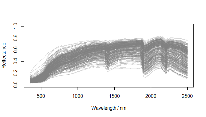
Raw reflectance spectra (datsoilspc$spc)
datsoilspc$spcA <- log(1 / as.matrix(datsoilspc$spc))

matplot(
  x = as.numeric(colnames(datsoilspc$spcA)),
  y = t(datsoilspc$spcA),
  xlab = "Wavelength / nm",
  ylab = "Absorbance",
  ylim = c(0, 4),
  type = "l",
  lty = 1,
  col = rgb(0.5, 0.5, 0.5, alpha = 0.3)
)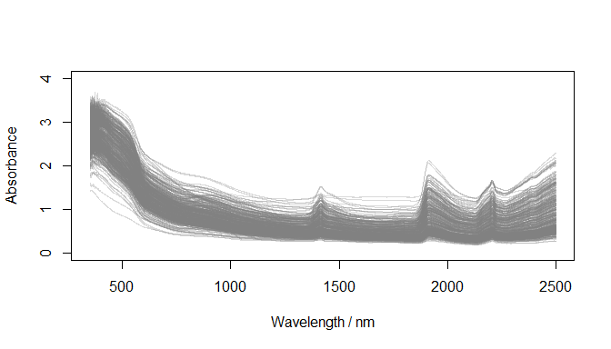
Absorbance spectra (datsoilspc$spcA)
oldWavs <- as.numeric(colnames(datsoilspc$spcA))
newWavs <- seq(min(oldWavs), max(oldWavs), by = 5)

datsoilspc$spcARs <- prospectr::resample(
  X = datsoilspc$spcA,
  wav = oldWavs,
  new.wav = newWavs,
  interpol = "linear"
)

datsoilspc$spcASnv <- prospectr::standardNormalVariate(datsoilspc$spcARs)
datsoilspc$spcAMovav <- prospectr::movav(datsoilspc$spcASnv, w = 11)

wavs <- as.numeric(colnames(datsoilspc$spcAMovav))

matplot(
  x = wavs,
  y = t(datsoilspc$spcAMovav),
  xlab = "Wavelength / nm",
  ylab = "Absorbance (SNV + movav)",
  type = "l",
  lty = 1,
  col = rgb(0.5, 0.5, 0.5, alpha = 0.3)
)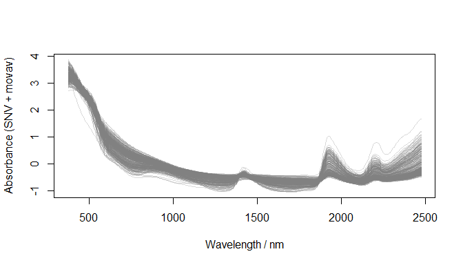
Preprocessed spectra (datsoilspc$spcAMovav)
set.seed(19101991)

calId <- sample(seq_len(nrow(datsoilspc)), size = round(0.75 * nrow(datsoilspc)))
datC <- datsoilspc[calId, ]
datV <- datsoilspc[-calId, ]  # <-- TEST

par(mfrow = c(1, 2))
hist(datC$TotalCarbon, main = "Calibration (datC)", xlab = "Total carbon")
hist(datV$TotalCarbon, main = "TEST (datV)", xlab = "Total carbon")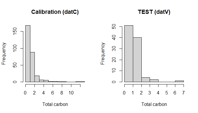
Calibration vs TEST splits (datC vs datV)
par(mfrow = c(1, 1))We fit PLS on calibration and evaluate on validation.
maxc <- 30

soilCPlsModel <- pls::plsr(
  TotalCarbon ~ spcAMovav,
  data = datC,
  method = "oscorespls",
  ncomp = maxc,
  validation = "CV"
)

plot(soilCPlsModel, "val", main = "PLS CV performance (datC)", xlab = "Number of components")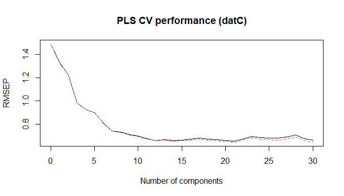
PLS CV performance (datC)
nc = 14).nc <- 14
# Refit on full datC with chosen nc (PLS itself uses all comps up to maxc; prediction uses nc)
soilCPlsPred_C <- as.numeric(predict(soilCPlsModel, ncomp = nc, newdata = datC$spcAMovav))
soilCPlsPred_T <- as.numeric(predict(soilCPlsModel, ncomp = nc, newdata = datV$spcAMovav))
par(mfrow = c(1, 2))
plot(datC$TotalCarbon, soilCPlsPred_C, xlab="Observed", ylab="Predicted", main="PLS (datC)", pch=16); abline(0,1)
plot(datV$TotalCarbon, soilCPlsPred_T, xlab="Observed", ylab="Predicted", main="PLS (TEST datV)", pch=16); abline(0,1)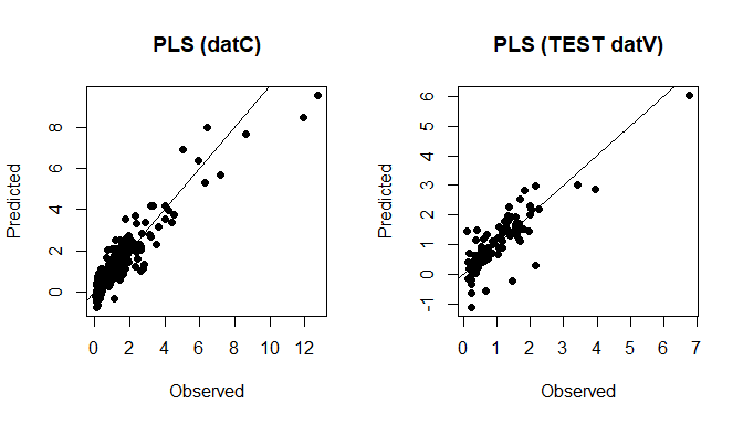
PLS predictions (datC + datV)
par(mfrow = c(1, 1))We use the same evaluation function used in many soilspec workflows.
pls_cal <- eval_quant(datC$TotalCarbon, soilCPlsPred_C)
pls_tst <- eval_quant(datV$TotalCarbon, soilCPlsPred_T)

as_df_metrics(pls_cal)
#>     n ME  MAE RMSE   R2 RPIQ  RPD
#> 1 293  0 0.37 0.56 0.86 2.04 2.63
as_df_metrics(pls_tst)
#>    n   ME  MAE RMSE   R2 RPIQ  RPD
#> 1 98 0.02 0.36 0.52 0.69 2.34 1.81This chunk detects if Python + TensorFlow + Keras can be
loaded.
If not available, the VAE section is skipped (vignette still
builds).
has_py <- reticulate::py_available(initialize = FALSE)

has_tf <- FALSE
if (has_py) {
  try(reticulate::py_config(), silent = TRUE)
  has_tf <- reticulate::py_module_available("tensorflow") &&
            reticulate::py_module_available("keras")
}

has_py
#> [1] TRUE
has_tf
#> [1] TRUE
Prepare Train/Val internal split within datC (no y transform; scale X only)
set.seed(19101991)

nC <- nrow(datC)
id_tr <- sample(seq_len(nC), size = round(0.80 * nC))
datC_tr <- datC[id_tr, ]
datC_va <- datC[-id_tr, ]

# y stays in original units (no transformation)
y_tr <- as.numeric(datC_tr$TotalCarbon)
y_va <- as.numeric(datC_va$TotalCarbon)

# X: scale predictors using TRAIN center/scale only
X_tr_raw <- as.matrix(datC_tr$spcAMovav)
X_va_raw <- as.matrix(datC_va$spcAMovav)
X_te_raw <- as.matrix(datV$spcAMovav)   # TEST

X_tr <- scale(X_tr_raw)
X_center <- attr(X_tr, "scaled:center")
X_scale  <- attr(X_tr, "scaled:scale")

# safe scaling: avoid division by zero
X_scale[X_scale == 0] <- 1

X_va <- scale(X_va_raw, center = X_center, scale = X_scale)
X_te <- scale(X_te_raw, center = X_center, scale = X_scale)

# sanity checks (dims)
dim(X_tr)
#> [1] 234 421
length(y_tr)
#> [1] 234
dim(X_va)
#> [1]  59 421
length(y_va)
#> [1] 59
dim(X_te)
#> [1]  98 421
Prepare Train/Val internal split within datC (no y transform; scale X only)
We model TotalCarbon using the preprocessed spectra
matrix spcAMovav.
reticulate::py_run_string("
import os
import random
import numpy as np
import tensorflow as tf

os.environ['PYTHONHASHSEED'] = '0'
random.seed(19101991)
np.random.seed(19101991)
tf.random.set_seed(19101991)
")

Sys.setenv(TF_DETERMINISTIC_OPS = "1")
Sys.setenv(TF_CPP_MIN_LOG_LEVEL = "2")         # reduce logs INFO/WARN
# Sys.setenv(TF_ENABLE_ONEDNN_OPTS = "0")

if (!has_tf) {
  message("TensorFlow/Keras not available; skipping soilVAE section.")
} else {

  Sys.setenv(TF_ENABLE_ONEDNN_OPTS="0")

  # Optional: force a specific python/venv/conda, if needed.
  # soilVAE::vae_configure(conda = "soilvae-tf")

  grid_vae <- data.frame(
    latent_dim = c(8L, 16L, 32L, 64L),
    dropout    = c(0.20, 0.30),
    lr         = c(5e-4),
    beta_kl    = c(0.01),
    alpha_y    = c(5),
    epochs     = c(500L),
    batch_size = c(64L, 128L),
    patience   = c(50L),
    stringsAsFactors = FALSE
  )

  grid_vae$hidden_enc <- list(c(512L, 256L, 128L))
  grid_vae$hidden_dec <- list(c(128L, 256L, 512L))

  tuned <- soilVAE::tune_vae_train_val(
    X_tr = X_tr, y_tr = y_tr,
    X_va = X_va, y_va = y_va,
    seed = 19101991,
    grid_vae = grid_vae
  )

  best <- soilVAE::select_best_from_grid(tuned$tuning_df, selection_metric = "euclid")

  cfg <- best$best

  # Refit on full datC (train+val) using early stopping monitored on the internal val (datC_va)
  m_vae <- soilVAE::vae_build(
    input_dim  = ncol(X_tr),
    hidden_enc = as.integer(strsplit(cfg$hidden_enc_str, "-")[[1]]),
    hidden_dec = as.integer(strsplit(cfg$hidden_dec_str, "-")[[1]]),
    latent_dim = as.integer(cfg$latent_dim),
    dropout    = as.numeric(cfg$dropout),
    lr         = as.numeric(cfg$lr),
    beta_kl    = as.numeric(cfg$beta_kl),
    alpha_y    = as.numeric(cfg$alpha_y)
  )

  soilVAE::vae_fit(
    model = m_vae,
    X = X_tr, y = y_tr,
    X_val = X_va, y_val = y_va,
    epochs = as.integer(cfg$epochs),
    batch_size = as.integer(cfg$batch_size),
    patience = as.integer(cfg$patience),
    verbose = 0L
  )

  yhat_tr <- as.numeric(soilVAE::vae_predict(m_vae, X_tr))
  yhat_va <- as.numeric(soilVAE::vae_predict(m_vae, X_va))
  yhat_te <- as.numeric(soilVAE::vae_predict(m_vae, X_te))

  # Metrics: internal train/val + FINAL TEST
  vae_trn <- eval_quant(y_tr, yhat_tr)
  vae_val <- eval_quant(y_va, yhat_va)
  vae_tst <- eval_quant(as.numeric(datV$TotalCarbon), yhat_te)

  # Plots
  par(mfrow = c(1, 3))
  plot(y_tr, yhat_tr, main="soilVAE (Train)", xlab="Observed", ylab="Predicted", pch=16); abline(0,1)
  plot(y_va, yhat_va, main="soilVAE (Val)",   xlab="Observed", ylab="Predicted", pch=16); abline(0,1)
  plot(as.numeric(datV$TotalCarbon), yhat_te, main="soilVAE (TEST datV)", xlab="Observed", ylab="Predicted", pch=16); abline(0,1)
  par(mfrow = c(1, 1))
}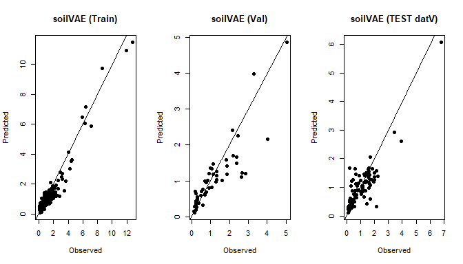
Train/Val splits for soilVAE
We present a compact comparison table.
if (!has_tf) {

  tab <- rbind(
    cbind(Model = "PLS", Split = "Calibration (datC)", as_df_metrics(pls_cal)),
    cbind(Model = "PLS", Split = "TEST (datV)",        as_df_metrics(pls_tst))
  )

} else {

  tab <- rbind(
    cbind(Model = "PLS",    Split = "Calibration (datC)", as_df_metrics(pls_cal)),
    cbind(Model = "PLS",    Split = "TEST (datV)",        as_df_metrics(pls_tst)),
    cbind(Model = "soilVAE",Split = "Train (internal)",   as_df_metrics(vae_trn)),
    cbind(Model = "soilVAE",Split = "Val (internal)",     as_df_metrics(vae_val)),
    cbind(Model = "soilVAE",Split = "TEST (datV)",        as_df_metrics(vae_tst))
  )

}

row.names(tab) <- NULL
tab
#>     Model              Split   n    ME  MAE RMSE   R2 RPIQ  RPD
#> 1     PLS Calibration (datC) 293  0.00 0.37 0.56 0.86 2.04 2.63
#> 2     PLS        TEST (datV)  98  0.02 0.36 0.52 0.69 2.34 1.81
#> 3 soilVAE   Train (internal) 234 -0.07 0.31 0.44 0.92 2.54 3.60
#> 4 soilVAE     Val (internal)  59 -0.10 0.33 0.51 0.76 2.36 2.04
#> 5 soilVAE        TEST (datV)  98 -0.04 0.33 0.47 0.74 2.56 1.97
If TensorFlow/Keras was not available, you can still use the PLS section and install a compatible Python stack later.
The PLS workflow depends only on R packages pls and
prospectr.
The supervised VAE requires:
-   Python (\>= 3.9)

-   TensorFlow (\>= 2.13)

- Keras (\>= 3)Education without ethics is only rhetoric.
Power without reflection is violence