![]()
SEMinRExtras adds functionality to the SEMinR package.
SEMinR (Ray, Danks, & Calero Valdez, 2026) is a domain specific language for modeling and estimating structural equation models. This is a supplementary package for SEMinR and not a standalone package. This package serves to provide additional extra methods and functions that can be used to analyze PLS-SEM models.
SEMinRExtras provides advanced SEM tools which are compatible with SEMinR. It implements several methods for evaluating and validating PLS-SEM models:
SEMinRExtras also serves to host the example models used in the PLS-SEM in R workbook (Hair et al., 2026).
| Function | Description |
|---|---|
assess_cvpat() |
CVPAT against LM and IA benchmarks |
assess_cvpat_compare() |
Compare predictive loss of two PLS models |
assess_pcm() |
Predictive Contribution of the Mediator (Danks, 2021) |
assess_ipma() |
Importance-Performance Map Analysis (IPMA) |
assess_cipma() |
Combined IPMA with Necessary Condition Analysis (cIPMA) |
assess_coa() |
Composite Overfit Analysis (full pipeline) |
predictive_deviance() |
Compute predictive deviance scores |
deviance_tree() |
Identify deviant case groups via decision tree |
unstable_params() |
Parameter instability analysis |
group_rules() |
Extract decision rules for deviant groups |
competes() |
Show competing splits at tree nodes |
assess_nca() |
Necessary Condition Analysis for PLS-SEM |
assess_nca_esse() |
NCA with Effect Size Sensitivity Extension |
assess_cta() |
Confirmatory Tetrad Analysis (CTA-PLS) with indicator borrowing (Gudergan et al., 2008) |
assess_fimix() |
FIMIX-PLS latent class segmentation |
assess_fimix_compare() |
Compare FIMIX solutions across K values |
assess_pos() |
PLS-POS prediction-oriented segmentation (Becker et al., 2013) |
assess_pos_compare() |
Compare PLS-POS solutions across K values |
pos_segments() |
Extract segment-specific re-estimated PLS models |
congruence_test() |
Bootstrapped congruence coefficient testing |
In order to access the demo files for the textbook, you can run the
demo() function after loading the SEMinRExtras package.
E.g.
demo("seminr-help-debugging", package = "seminrExtras")
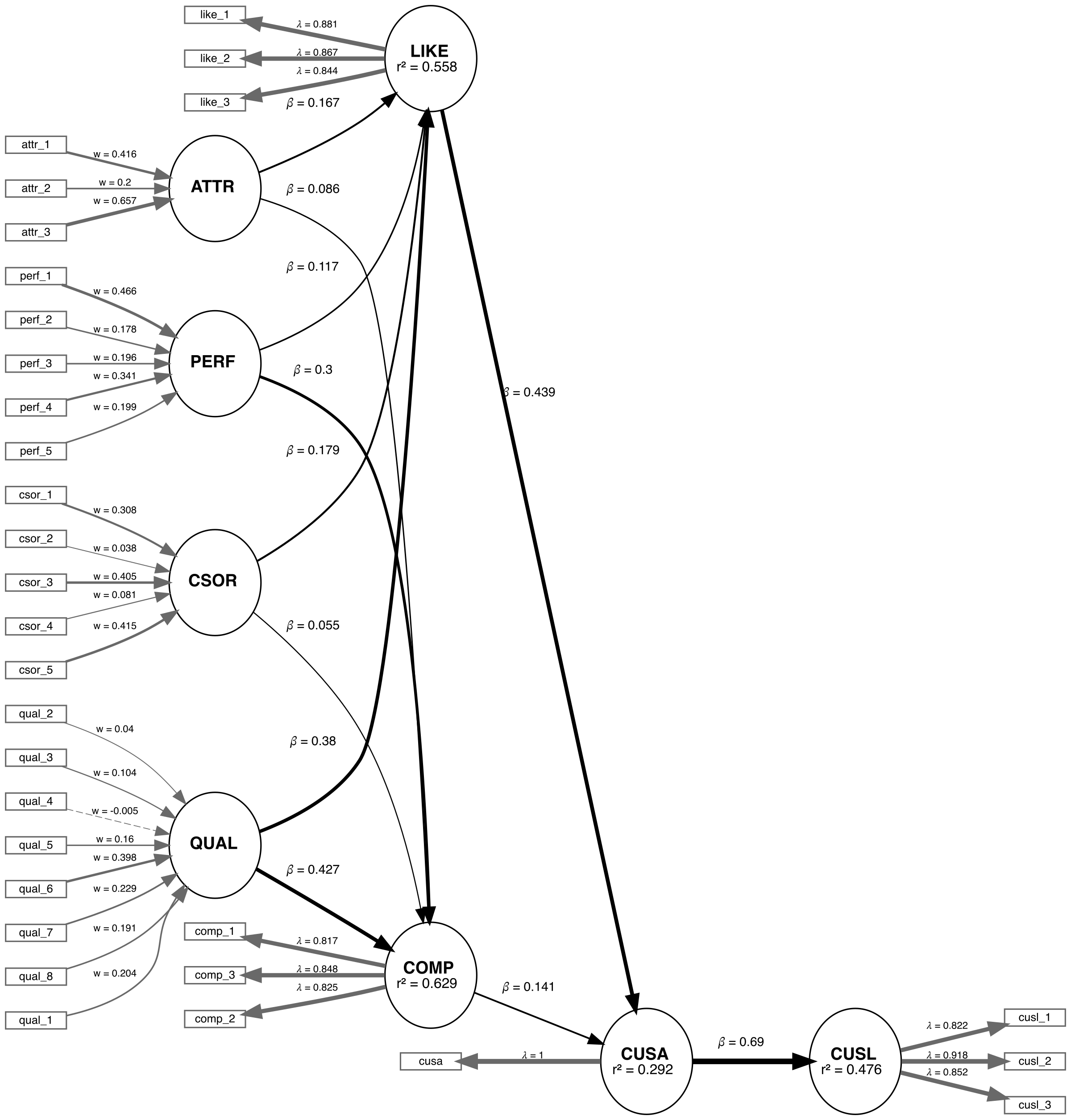
We are applying the CVPAT process to the corporate reputation example bundled with SEMinR. Since we will be comparing two models, we will first estimate and plot both models. Below you will find the competing and established models which will be compared.
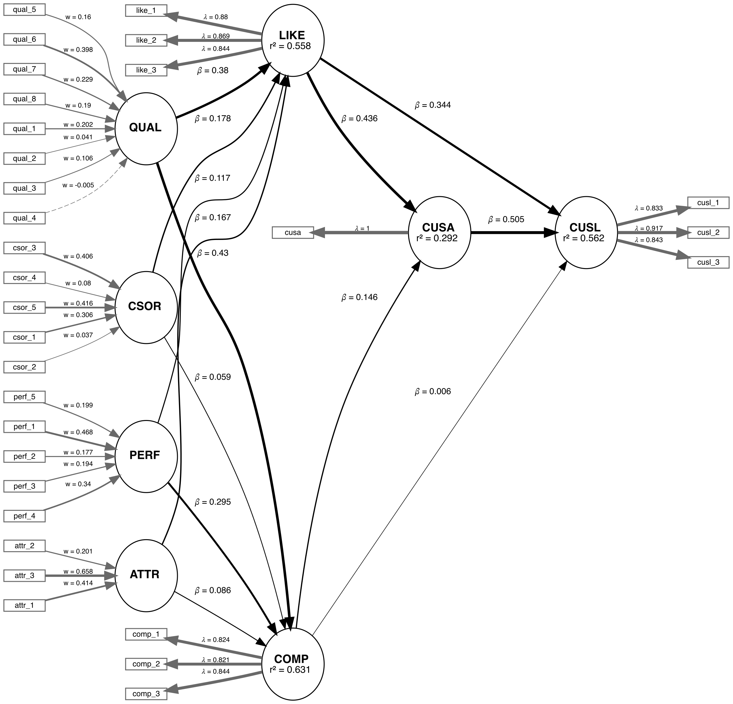
# Create measurement model ----
corp_rep_mm_ext <- constructs(
  composite("QUAL", multi_items("qual_", 1:8), weights = mode_B),
  composite("PERF", multi_items("perf_", 1:5), weights = mode_B),
  composite("CSOR", multi_items("csor_", 1:5), weights = mode_B),
  composite("ATTR", multi_items("attr_", 1:3), weights = mode_B),
  composite("COMP", multi_items("comp_", 1:3)),
  composite("LIKE", multi_items("like_", 1:3)),
  composite("CUSA", single_item("cusa")),
  composite("CUSL", multi_items("cusl_", 1:3))
)

alt_mm <- constructs(
  composite("QUAL", multi_items("qual_", 1:8), weights = mode_B),
  composite("PERF", multi_items("perf_", 1:5), weights = mode_B),
  composite("CSOR", multi_items("csor_", 1:5), weights = mode_B),
  composite("ATTR", multi_items("attr_", 1:3), weights = mode_B),
  composite("COMP", multi_items("comp_", 1:3)),
  composite("LIKE", multi_items("like_", 1:3)),
  composite("CUSA", single_item("cusa")),
  composite("CUSL", multi_items("cusl_", 1:3))
)

# Create structural model ----
corp_rep_sm_ext <- relationships(
  paths(from = c("QUAL", "PERF", "CSOR", "ATTR"), to = c("COMP", "LIKE")),
  paths(from = c("COMP", "LIKE"), to = c("CUSA", "CUSL")),
  paths(from = c("CUSA"),         to = c("CUSL"))
)
alt_sm <- relationships(
  paths(from = c("QUAL", "PERF", "CSOR", "ATTR"), to = c("COMP", "LIKE")),
  paths(from = c("COMP", "LIKE"), to = c("CUSA")),
  paths(from = c("CUSA"),         to = c("CUSL"))
)


# Estimate the models ----
established_model <- estimate_pls(
  data = corp_rep_data,
  measurement_model = corp_rep_mm_ext,
  structural_model  = corp_rep_sm_ext,
  missing = mean_replacement,
  missing_value = "-99")

competing_model <- estimate_pls(
  data = corp_rep_data,
  measurement_model = alt_mm,
  structural_model  = alt_sm,
  missing = mean_replacement,
  missing_value = "-99")

# Function to compare the Loss of two models
compare_results <- assess_cvpat_compare(established_model = established_model,
                                        alternative_model = competing_model,
                                        testtype = "two.sided",
                                        nboot = 2000,
                                        technique = predict_DA,
                                        seed = 123,
                                        noFolds = 10,
                                        reps = 10,
                                        cores = 1)


print(compare_results,
      digits = 3)

# Assess the base model ----
assess_results <- assess_cvpat(established_model,
                               seed = 123,
                               cores = 1)
print(assess_results$CVPAT_compare_LM,
      digits = 3)
print(assess_results$CVPAT_compare_IA,
digits = 3)# Assess the base model ----
assess_results <- assess_cvpat(established_model,
seed = 123,
cores = 1)
print(assess_results$CVPAT_compare_LM,
digits = 3)
#> PLS Loss LM Loss Diff Boot T value Boot P Value
#> COMP 1.196 1.211 -0.015 0.542 0.588
#> LIKE 1.915 2.063 -0.148 3.761 0.000
#> CUSA 0.994 0.983 0.011 -0.489 0.625
#> CUSL 1.560 1.600 -0.040 2.914 0.004
#> Overall 1.416 1.464 -0.048 3.482 0.001
#>
#> CVPAT as per Sharma et al. (2023).
print(assess_results$CVPAT_compare_IA,
digits = 3)
#> PLS Loss IA Loss Diff Boot T value Boot P Value
#> COMP 1.196 2.023 -0.827 8.580 0.000
#> LIKE 1.915 3.103 -1.187 8.293 0.000
#> CUSA 0.994 1.374 -0.379 5.004 0.000
#> CUSL 1.560 2.663 -1.102 7.572 0.000
#> Overall 1.416 2.290 -0.874 10.301 0.000
#>
#> CVPAT as per Sharma et al. (2023).The established model has significantly lower predictive loss compared to both the naive benchmark IA and the LM model. Thus, we can say that the established model has predictive relevance.
Now we compare the results:
# Function to compare the Loss of two models
compare_results <- assess_cvpat_compare(established_model = established_model,
                                        alternative_model = competing_model,
                                        testtype = "two.sided",
                                        nboot = 2000,
                                        technique = predict_DA,
                                        seed = 123,
                                        noFolds = 10,
                                        reps = 10,
                                        cores = 1)

print(compare_results,
      digits = 3)
#>         Base Model Loss Alt Model Loss   Diff Boot T value Boot P Value
#> COMP              1.198          1.195  0.003       -0.460        0.645
#> LIKE              1.923          1.933 -0.010        0.883        0.378
#> CUSA              0.988          0.992 -0.004        0.809        0.419
#> CUSL              1.562          1.715 -0.152        3.286        0.001
#> Overall           1.418          1.459 -0.041        3.293        0.001
#>
#> CVPAT as per Sharma, Liengaard, Hair, Sarstedt, & Ringle, (2023).
#>   Both models under comparison have identical endogenous constructs with identical measurement models.
#>   Purely exogenous constructs can differ in regards to their relationships with both nomological
#>   partners and measurement indicators.
The established model has significantly lower predictive loss compared to the competing model. Thus, we can say that the established model has superior predictive performance compared to the competing model.
CTA-PLS (Gudergan et al., 2008) empirically tests whether a construct’s measurement model is consistent with a reflective (common factor) specification. Under a reflective model, all model-implied vanishing tetrads equal zero. If any tetrad is significantly non-zero, the reflective specification is rejected in favour of a formative one.
CTA-PLS requires at least 4 indicators per construct. When
borrow = TRUE (the default), constructs with only 2 or 3
indicators can still be tested by borrowing indicators from structurally
connected constructs. The borrowing rules follow Gudergan et al. (2008,
Table 1): a reflective construct with 3 own indicators borrows 1 from an
adjacent reflective construct (all tetrads vanish under H0), while a
construct with 2 own indicators borrows 2 from any adjacent construct
(only the cross-tetrad tau_1342 vanishes).
library(seminr)
library(seminrExtras)

mobi_mm <- constructs(
  composite("Image",        multi_items("IMAG", 1:5)),
  composite("Expectation",  multi_items("CUEX", 1:3)),
  composite("Value",        multi_items("PERV", 1:2)),
  composite("Satisfaction", multi_items("CUSA", 1:3)),
  composite("Loyalty",      multi_items("CUSL", 1:3))
)

mobi_sm <- relationships(
  paths(from = "Image",       to = c("Expectation", "Satisfaction", "Loyalty")),
  paths(from = "Expectation", to = c("Value", "Satisfaction")),
  paths(from = "Value",       to = "Satisfaction"),
  paths(from = "Satisfaction", to = "Loyalty")
)

mobi_pls <- estimate_pls(data = mobi,
                          measurement_model = mobi_mm,
                          structural_model  = mobi_sm)

# CTA-PLS with borrowing (default) — constructs with 2-3 indicators
# borrow from adjacent constructs to form testable 4-tuples
cta_result <- assess_cta(mobi_pls, nboot = 5000, seed = 123)
print(cta_result)
summary(cta_result)

# Without borrowing — only constructs with >= 4 indicators are tested
cta_no_borrow <- assess_cta(mobi_pls, nboot = 5000, borrow = FALSE)
print(cta_no_borrow)FIMIX-PLS and PLS-POS are complementary approaches for detecting unobserved heterogeneity in PLS-SEM. FIMIX-PLS uses probabilistic (EM-based) assignment and assumes normally distributed residuals, while PLS-POS uses deterministic (hill-climbing) assignment with no distributional assumptions. Both methods partition the sample into K segments with segment-specific path coefficients.
FIMIX-PLS (Hahn et al., 2002; Sarstedt et al., 2011) probabilistically assigns observations to K segments, each with segment-specific structural path coefficients.
assess_fimix() estimates a single K-segment solution,
while assess_fimix_compare() compares solutions across K
values using information criteria (AIC, BIC, CAIC, etc.) to help select
the optimal number of segments.
library(seminr)
library(seminrExtras)

# Estimate a PLS model
corp_pls <- estimate_pls(
  data = corp_rep_data,
  measurement_model = corp_rep_mm_ext,
  structural_model  = corp_rep_sm_ext,
  missing = mean_replacement,
  missing_value = "-99")

# FIMIX with K=2 segments
fimix_k2 <- assess_fimix(corp_pls, K = 2, nstart = 10, seed = 123)
print(fimix_k2)
summary(fimix_k2)
plot(fimix_k2)

# Compare across K=2..4 using information criteria
fimix_compare <- assess_fimix_compare(corp_pls,
                                       K_range = 2:4,
                                       nstart = 10,
                                       seed = 123)
print(fimix_compare)
plot(fimix_compare)
PLS-POS (Becker et al., 2013) maximizes the sum of R-squared across all endogenous constructs across K segments using deterministic hill-climbing. Unlike FIMIX-PLS, it makes no distributional assumptions and can detect heterogeneity in both structural and formative measurement models.
assess_pos() estimates a single K-segment solution,
while assess_pos_compare() compares solutions across
multiple K values using the objective criterion (sum of R-squared).
# PLS-POS with K=2 segments (using corp_pls from above)
pos_k2 <- assess_pos(corp_pls, K = 2, nstart = 10, seed = 123)
print(pos_k2)
summary(pos_k2)
plot(pos_k2, type = "rsquared")

# Compare across K=2..4
pos_compare <- assess_pos_compare(corp_pls,
                                   K_range = 2:4,
                                   nstart = 10,
                                   seed = 123)
print(pos_compare)
plot(pos_compare)
Congruence testing (Franke, Sarstedt, & Danks, 2021) evaluates whether PLS composite weights are stable across bootstrap samples by computing congruence coefficients. A congruence coefficient close to 1 indicates that the composite weight pattern is robust.
cong_result <- congruence_test(mobi_pls,
                                nboot = 2000,
                                seed = 123)
print(cong_result)
summary(cong_result)