Help for package oce

Title:

Analysis of Oceanographic Data

Version:

1.8-3

Maintainer:

Dan Kelley <Dan.Kelley@Dal.Ca>

Depends:

R (≥ 4.1.0), gsw, methods, utils

Suggests:

automap, DBI, foreign, interp, knitr, lubridate, ncdf4, ocedata, rmarkdown, RSQLite, R.utils, sf, terra, testthat (≥ 3.0.0), tiff, XML

BugReports:

https://github.com/dankelley/oce/issues

Description:

Supports the analysis of Oceanographic data, including 'ADCP' measurements, measurements made with 'argo' floats, 'CTD' measurements, sectional data, sea-level time series, coastline and topographic data, etc. Provides specialized functions for calculating seawater properties such as potential temperature in either the 'UNESCO' or 'TEOS-10' equation of state. Produces graphical displays that conform to the conventions of the Oceanographic literature. This package is discussed extensively by Kelley (2018) "Oceanographic Analysis with R" <doi:10.1007/978-1-4939-8844-0>.

License:

GPL-2 | GPL-3 [expanded from: GPL (≥ 2)]

Encoding:

UTF-8

URL:

https://dankelley.github.io/oce/

LazyData:

false

RoxygenNote:

7.3.2

BuildVignettes:

true

VignetteBuilder:

knitr

NeedsCompilation:

yes

LinkingTo:

Rcpp

Imports:

Rcpp

Packaged:

2024-08-17 09:38:38 UTC; kelley

Config/testthat/edition:

Author:

Dan Kelley

[aut, cre], Clark Richards

[aut], Chantelle Layton

[ctb] (curl() coauthor), British Geological Survey [ctb, cph] (magnetic-field subroutine)

Repository:

CRAN

Date/Publication:

2024-08-17 10:20:04 UTC

A Package for Oceanographic Analysis

Description

The oce package provides functions for working with Oceanographic data, for calculations that are specific to Oceanography, and for producing graphics that match the conventions of the field.

Details

Over a dozen specialized data types are handled by oce, with generic plots and summaries for each, along with the specialized functions needed for typical Oceanographic analysis.

See oce for a summary of the class structure and links to documentation for the many subclasses of oce objects, each aligned with a class of instrument or or type of dataset. For a more task-oriented approach, see the several vignettes that are provided with oce, and a book (Kelley, Dan E. Oceanographic Analysis with R. New York: Springer-Verlag, 2018. https://link.springer.com/book/10.1007/978-1-4939-8844-0) written by one of the oce co-authors.

Specialized Functions

A key function is read.oce(), which will attempt to read Oceanographic data in raw format. This uses oceMagic() to try to detect the file type, based on the file name and contents. If this detection is not possible, users will need to go beyond read.oce(), using a more specialized function, e.g. read.ctd() for CTD files, read.ctd.sbe() for Teledyne-Seabird files, etc.

Generic Methods

A list of the generic methods in oce is provided by methods(class="oce"); a few that are used frequently are as follows.

[[ Finds the value of an item in the object's metadata or data slot. If the item does not exist, but can be calculated from the other items, then the calculated value is returned. As an example of the latter, consider the built-in ctd dataset, which does not contain potential temperature, "theta". Using ctd[["theta"]] therefore causes swTheta() to be called, to calculate theta. See [[,oce-method or type ?"[[,oce-method" to learn more about general functioning, or a specialized method like [[,ctd-method for CTD data, etc.
⁠[[<-⁠ Alters the named item in the object's metadata or data slot. If the item does not exist, it is created. See [[<-,oce-method or type ?"[[<-,oce-method" to learn more about the general methodology, or a specialized method like [[<-,ctd-method for CTD data, etc.
summary() Displays some information about the object named as an argument, including a few elements from its metadata slot and some statistics of the contents of its data slot. See summary,oce-method or type ?"summary,oce-method" to learn more about general functioning, or a specialized method like summary,ctd-method for CTD data, etc.
subset() Takes a subset of an oce object. See subset,oce-method or type ?"subset,oce-method" to learn more about general functioning, or a specialized method like subset,ctd-method for CTD data, etc.

Author(s)

Maintainer: Dan Kelley Dan.Kelley@Dal.Ca (ORCID)

Authors:

Clark Richards clark.richards@gmail.com (ORCID)

Other contributors:

Chantelle Layton chantelle.layton@dal.ca (ORCID) (curl() coauthor) [contributor]
British Geological Survey (magnetic-field subroutine) [contributor, copyright holder]

Sample ctd File in .odf Format

Description

The location is approximately 30km southeast of Halifax Harbour, at "Station 2" of the Halifax Line on the Scotian Shelf.

Examples

ctd <- read.ctd(system.file("extdata", "CTD_BCD2014666_008_1_DN.ODF.gz", package="oce"))
plot(ctd)

Determine Time Offset From Timezone

Description

The data are from ⁠https://www.timeanddate.com/time/zones/⁠ and were hand-edited to develop this code, so there may be errors. Also, note that some of these contradict; if you examine the code, you'll see some commented-out portions that represent solving conflicting definitions by choosing the more common timezone abbreviation over a the less common one.

Usage

GMTOffsetFromTz(tz)

Arguments

tz

a timezone, e.g. UTC.

Value

Number of hours in offset, e.g. AST yields 4.

Author(s)

Dan Kelley

Examples

library(oce)
cat("Atlantic Standard Time is ", GMTOffsetFromTz("AST"), "hours after UTC")

Create ODF Object From Output of read_ODF in ODF package

Description

As of August 11, 2015, ODF::read_ODF returns a list with 9 elements, one named DATA, which is a data.frame() containing the columnar data, the others being headers of various sorts. The present function constructs an oce object from such data, facilitating processing and plotting with the general oce functions. This involves storing the 8 headers verbatim in the odfHeaders in the metadata slot, and also copying some of the header information into more standard names (e.g. metadata@longitude is a copy of metadata@odfHeader$EVENT_HEADER$INITIAL_LATITUDE). As for the DATA, they are stored in the data slot, after renaming from ODF to oce convention using ODFNames2oceNames().

Usage

ODF2oce(ODF, coerce = TRUE, debug = getOption("oceDebug"))

Arguments

ODF

A list as returned by read_ODF in the ODF package

coerce

A logical value indicating whether to coerce the return value to an appropriate object type, if possible.

debug

a flag that turns on debugging. Set to 1 to get a moderate amount of debugging information, or to 2 to get more.

Value

An oce object, possibly coerced to a subtype.

Caution

This function may change as the ODF package changes. Since ODF has not been released yet, this should not affect any users except those involved in the development of oce and ODF.

Author(s)

Dan Kelley

Create a List of odf Header Metadata

Description

Create a List of odf Header Metadata

Usage

ODFListFromHeader(header)

Arguments

header

Vector of character strings, holding the header

Value

A list holding the metadata, with item names matching those in the ODF header, except that duplicates are transformed through the use of unduplicateNames().

Translate ODF CODE Strings to oce Variable Names

Description

Translate ODF CODE strings to oce variable names. This is done differently for data names and quality-control (QC) names.

Usage

ODFNames2oceNames(
  ODFnames,
  columns = NULL,
  PARAMETER_HEADER = NULL,
  debug = getOption("oceDebug")
)

Arguments

ODFnames

vector of character values that hold ODF names.

columns

Optional list containing name correspondances, as described for read.ctd.odf().

PARAMETER_HEADER

Optional list containing information on the data variables.

debug

an integer specifying whether debugging information is to be printed during the processing. This is a general parameter that is used by many oce functions. Generally, setting debug=0 turns off the printing, while higher values suggest that more information be printed. If one function calls another, it usually reduces the value of debug first, so that a user can often obtain deeper debugging by specifying higher debug values.

Details

The following table gives the recognized ODF code names for variables, along with the translated names as used in oce objects. Note that the code names are appended with strings such as "_01", "_02", etc, for repeats. The converted name for an "_01" item is as shown below, and for e.g. "_02" a suffix 2 is added to the oce name, etc.

QC items (which get stored as flags in object's metadata slots) are assigned names that match those of the parameters to which they refer. In parsing ODF files, it is assumed that QC items refer to the data items that precede them. This pattern does not seem to be documented, but it has held in all the files examined by the author, and a similar assumption is made in other software systems. QC items have CODE values that are either start with "QQQQ" or equal "Q<CODE>", where ⁠<CODE>⁠ matches the corresponding data item.

ODF Code	Oce Name	Notes
`ABSH`	`humidityAbsolute`
`ACO2`	`CO2Atmosphere`
`ALKW`	`alkalinity`
`ALKY`	`alkalinityTotal`
`ALP0`	`apha0`
`ALTB`	`altimeter`
`ALTS`	`altitude`
`AMON`	`ammonium`
`ATMP`	`pressureAtmosphere`
`ATMS`	`pressureAtmosphereSealevel`
`ATRK`	`alongTrackDisplacement`
`ATTU`	`attenuation`
`AUTH`	`authority`
`BATH`	`barometricDepth`
`BATT`	`batteryVoltage`
`BEAM`	`a`
`BNO7`	`bestNODC7Number`	That is an "oh" letter, not a zero
`CALK`	`carbonateAlkalinity`
`CHLR`	`chlorinity`
`CHLS`	`chlorosity`
`CNDC`	`conductivity`
`CNTR`	`scan`
`COND`	`conductivity`
`CORG`	`carbonOrganic`
`CPHL`	`chlorophyll`
`CRAT`	`conductivity`	Conductivity ratio (may have spurious unit)
`CMNT`	`comment`
`CNDC`	`conductivity`
`COND`	`conductivity`
`CTOT`	`carbonTotal`
`DCHG`	`discharge`
`DENS`	`density`
`DEPH`	`pressure`
`DEWT`	`temperatureDewpoint`
`DOC_`	`carbonOrganicDissolved`
`DON_`	`nitrogenOrganicDissolved`
`DOXY`	`oxygen`
`DPDT`	`dpdt`
`DRDP`	`drogueDepth`
`DPWT`	`dryWeight`
`DRYT`	`temperatureDryBulb`
`DYNH`	`dynamicHeight`
`ERRV`	`errorVelocity`
`EWCM`	`uMagnetic`
`EWCT`	`u`
`FFFF`	`overall(FFFF)`	Archaic overall flag, replaced by `QCFF`
`FLOR`	`fluorometer`
`GDIR`	`windDirectionGust`
`GEOP`	`geopotential`
`GSPD`	`windSpeedGust`
`HCDM`	`directionMagnetic`
`HCDT`	`directionTrue`
`HCSP`	`speedHorizontal`
`HEAD`	`heading`
`HSUL`	`hydrogenSulphide`
`IDEN`	`sampleNumber`
`LABT`	`temperatureLaboratory`
`LATD`	`latitude`
`LHIS`	`lifeHistory`
`LOND`	`longitude`
`LPHT`	`pHLaboratory`
`MNSV`	`retentionFilterSize`
`MNSZ`	`organismSizeMinimum`
`MODF`	`additionalTaxonomicInformation`
`MXSZ`	`organismSizeMaximum`
`NETR`	`netSolarRadiation`
`NONE`	`noWMOcode`
`NORG`	`nitrogenOrganic`
`NSCM`	`vMagnetic`
`NSCT`	`v`
`NTOT`	`nitrogenTotal`
`NTRA`	`nitrate`
`NTRI`	`nitrite`
`NTRZ`	`nitrite+nitrate`
`NUM_`	`scansPerAverage`
`OBKS`	`turbidity`
`OCUR`	`oxygenCurrent`
`OPPR`	`oxygenPartialPressure`
`OSAT`	`oxygenSaturation`
`OTMP`	`oxygenTemperature`
`OXYG`	`oxygenDissolved`
`OXYM`	`oxygenDissolved`
`OXYV`	`oxygenVoltage`
`OXV_`	`oxygenVoltageRaw`
`PCO2`	`CO2`
`PHA_`	`phaeopigment`
`PHOS`	`phosphate`
`PHPH`	`pH`
`PHT_`	`pHTotal`
`PIM_`	`particulateInorganicMatter`
`PHY_`	`phytoplanktonCount`
`POC_`	`particulateOrganicCarbon`
`POM_`	`particulateOrganicMatter`
`PON_`	`particulateOrganicNitrogen`
`POTM`	`theta`
`PRES`	`pressure`
`PSAL`	`salinity`
`PSAR`	`PSAR`
`PTCH`	`pitch`
`QCFF`	`overall(QCFF)`	Overall flag (see also archaic FFFF)
`RANG`	`range`
`REFR`	`reference`
`RELH`	`humidityRelative`
`RELP`	`relativeTotalPressure`
`ROLL`	`roll`
`SDEV`	`standardDeviation`
`SECC`	`SecchiDepth`
`SEX_`	`sex`
`SIG0`	`sigma0`
`SIGP`	`sigmaTheta`
`SIGT`	`sigmat`
`SLCA`	`silicate`
`SNCN`	`scanCounter`
`SPAR`	`SPAR`
`SPEH`	`humiditySpecific`
`SPFR`	`sampleFraction`
`SPVO`	`specificVolume`
`SPVA`	`specificVolumeAnomaly`
`STRA`	`stressAmplitude`
`STRD`	`stressDirection`
`STRU`	`stressU`
`STRV`	`stressV`
`SSAL`	`salinity`
`SVEL`	`soundVelocity`
`SYTM`	`time`
`TAXN`	`taxonomicName`
`TE90`	`temperature`
`TEMP`	`temperature`
`TEXZT`	`text`
`TICW`	`totalInorganicCarbon`
`TILT`	`tilt`
`TOTP`	`pressureAbsolute`
`TPHS`	`phosphorousTotal`
`TRAN`	`lightTransmission`
`TRB_`	`turbidity`
`TRBH`	`trophicDescriptor`
`TSM_`	`suspendedMatterTotal`
`TSN_`	`taxonomicSerialNumber`
`TURB`	`turbidity`
`UNKN`	`-`
`UREA`	`urea`
`VAIS`	`BVFrequency`
`VCSP`	`w`
`VMXL`	`waveHeightMaximum`
`VRMS`	`waveHeightMean`
`VTCA`	`wavePeriod`
`WDIR`	`windDirection`
`WETT`	`temperatureWetBulb`
`WSPD`	`windSpeed`
`WTWT`	`wetWeight`
`ZOO_`	`zooplanktonCount`

Any code not shown in the list is transferred to the oce object without renaming, apart from the adjustment of suffix numbers. The following code have been seen in data files from the Bedford Institute of Oceanography: ALTB, PHPH and QCFF.

Value

A list relating ODF names to oce names (see “Examples”).

Author(s)

Dan Kelley

References

For sources that describe the ODF format, see the documentation for the odf.

Examples

ODFNames2oceNames("TEMP_01")$names # "temperature"

Convert From ITS-90 to IPTS-68 Temperature

Description

Today's instruments typically record in the ITS-90 scale, but some old datasets will be in the IPTS-68 scale. T90fromT68() converts from the IPTS-68 to the ITS-90 scale, using Saunders' (1990) formula, while T68fromT90() does the reverse. The difference between IPTS-68 and ITS-90 values is typically a few millidegrees (see ‘Examples’), which is seldom visible on a typical temperature profile, but may be of interest in some precise work. Mostly for historical interest, T90fromT48() is provided to convert from the ITS-48 system to ITS-90.

Usage

T68fromT90(temperature)

Arguments

temperature

numeric vector of temperatures]in ^\circC on the ITS-90 scale.

Value

Corresponding temperatures in ^\circC on the IPTS-68 scale.

Author(s)

Dan Kelley

References

P. M. Saunders, 1990. The international temperature scale of 1990, ITS-90. WOCE Newsletter, volume 10, September 1990, page 10. http://www.nodc.noaa.gov/woce/wdiu/wocedocs/newsltr/news10/contents.htm

Examples

library(oce)
T68 <- seq(3, 20, 1)
T90 <- T90fromT68(T68)
sqrt(mean((T68-T90)^2))

Convert From ITS-48 to ITS-90 Temperature

Description

Usage

T90fromT48(temperature)

Arguments

temperature

Vector of temperatures in ^\circC on the IPTS-48 scale.

Value

Corresponding temperatures in ^\circC on the ITS-90 scale.

Author(s)

Dan Kelley

References

P. M. Saunders, 1990. The international temperature scale of 1990, ITS-90. WOCE Newsletter, volume 10, September 1990, page 10. http://www.nodc.noaa.gov/woce/wdiu/wocedocs/newsltr/news10/contents.htm

Examples

library(oce)
T68 <- seq(3, 20, 1)
T90 <- T90fromT68(T68)
sqrt(mean((T68-T90)^2))

Convert From IPTS-68 to ITS-90 Temperature

Description

Usage

T90fromT68(temperature)

Arguments

temperature

numeric vector of temperatures in ^\circC on the IPTS-68 scale.

Value

Corresponding temperatures in ^\circC on the ITS-90 scale.

Author(s)

Dan Kelley

References

P. M. Saunders, 1990. The international temperature scale of 1990, ITS-90. WOCE Newsletter, volume 10, September 1990, page 10. http://www.nodc.noaa.gov/woce/wdiu/wocedocs/newsltr/news10/contents.htm

Examples

library(oce)
T68 <- seq(3, 20, 1)
T90 <- T90fromT68(T68)
sqrt(mean((T68-T90)^2))

Replace Parts of an adp Object

Description

In addition to the usual insertion of elements by name, note that e.g. pitch gets stored into pitchSlow.

The [[<- method works for all oce objects. The purpose, as with the related extraction method, [[, is to insulate users from the internal details of oce objects, by looking for items within the various storage slots of the object. Items not actually stored can also be replaced, including units and data-quality flags.

Usage

## S4 replacement method for signature 'adp'
x[[i, j, ...]] <- value

Arguments

x

an adp object.

i

character value naming the item to replace.

j

optional additional information on the i item.

...

optional additional information (ignored).

value

The value to be placed into x, somewhere.

Details

As with [[ method, the procedure works in steps.

First, the metadata slot of x is checked to see whether it contains something named with i. If so, then the named item is replaced with value.

Otherwise, if the string value of i ends in Unit, then the characters preceding that are taken as the name of a variable, and the metadata slot of x is updated to store that unit, e.g.

x[["temperatureUnits"]] <- list(unit=expression(degree*F),scale="")

Similarly, if i ends in Flag, then quality-control flags are set up as defined by result, e.g.

o[["temperatureFlags"]] <- c(2,4,2,2)

Otherwise, pmatch() is used for a partial-string match with the names of the items that are in the data slot of x. The first item found (if any) is then updated to hold the value result.

If none of these conditions is met, a warning is issued.

Author(s)

Dan Kelley

Replace Parts of an adv Object

Description

Generally, the [[ method lets users extract information from oce objects, without having to know the details of the internal storage. For many oce sub-classes, [[ can also return quantities that are computed from the object's contents.

Usage

## S4 replacement method for signature 'adv'
x[[i, j, ...]] <- value

Arguments

x

an adv object.

i

character value indicating the name of an item to extract.

j

optional additional information on the i item.

...

ignored.

value

The value to be inserted into x.

Details

If the adv object holds slow variables (i.e. if timeSlow is in the data slot), then assigning to .e.g. heading will not actually assign to a variable of that name, but instead assigns to headingSlow. To catch misapplication of this rule, an error message will be issued if the assigned value is not of the same length as timeSlow.

A two-step process is used to try to find the requested information. First, a class-specific function is used (see “Details of the Specialized Method”). If this yields nothing, then a general method is used (see “Details of the General Method”). If both methods fail, then [[ returns NULL.

Some understanding of the subclass is required to know what can be retrieved with [[. When dealing with an unfamiliar subclass, it can be useful to first use x[["?"]] to get a listing of the retrievable items. See “Details of the Specialized Method” for more information.

Details of the General Method

Note: the text of this section is identical for all oce subclasses, and so some of what you read here may not be relevant to the class being described in this help page.

If the specialized method produces no matches, the following generalized method is applied. As with the specialized method, the procedure hinges first on the values of i and, optionally, j. The work proceeds in steps, by testing a sequence of possible conditions in sequence.

A check is made as to whether i names one of the standard oce slots. If so, [[ returns the slot contents of that slot. Thus, x[["metadata"]] will retrieve the metadata slot, while x[["data"]] and x[["processingLog"]] return those slots.
If i is a string ending in the "Unit", then the characters preceding that string are taken to be the name of an item in the data object, and a list containing the unit is returned (or NULL if there is no such unit). This list consists of an item named unit, which is an expression(), and an item named scale, which is a string describing the measurement scale. If the string ends in " unit", e.g. x[["temperature unit"]] (note the space), then just the expression is returned, and if it ends in " scale", then just the scale is returned.
If i is a string ending in "Flag", then the corresponding data-quality flag is returned (or NULL if there is no such flag).
If the object holds hydrographic information (pressure, salinity, temperature, longitude and latitude) then another set of possibilities arises. If i is "sigmaTheta", then the value of swSigmaTheta() is called with x as the sole argument, and the results are returned. Similarly, swSigma0() is used if i="sigma0", and swSpice() is used if i="spice". Of course, these actions only make sense for objects that contain the relevant items within their data slot.
After these possibilities are eliminated, the action depends on whether j has been provided. If j is not provided, or is the string "", then i is sought in the metadata slot, and then in the data slot, returning whichever is found first. In other words, if j is not provided, the metadata slot takes preference over the data slot. However, if j is provided, then it must be either the string "metadata" or "data", and it directs where to look.
If none of the above-listed conditions holds, then NULL is returned.

Author(s)

Dan Kelley

Replace Parts of an amsr Object

Description

Usage

## S4 replacement method for signature 'amsr'
x[[i, j, ...]] <- value

Arguments

x

an amsr object.

i

character value naming the item to replace.

j

optional additional information on the i item.

...

optional additional information (ignored).

value

The value to be placed into x, somewhere.

Details

As with [[ method, the procedure works in steps.

First, the metadata slot of x is checked to see whether it contains something named with i. If so, then the named item is replaced with value.

Otherwise, if the string value of i ends in Unit, then the characters preceding that are taken as the name of a variable, and the metadata slot of x is updated to store that unit, e.g.

x[["temperatureUnits"]] <- list(unit=expression(degree*F),scale="")

Similarly, if i ends in Flag, then quality-control flags are set up as defined by result, e.g.

o[["temperatureFlags"]] <- c(2,4,2,2)

Otherwise, pmatch() is used for a partial-string match with the names of the items that are in the data slot of x. The first item found (if any) is then updated to hold the value result.

If none of these conditions is met, a warning is issued.

Replace Parts of an argo Object

Description

Usage

## S4 replacement method for signature 'argo'
x[[i, j, ...]] <- value

Arguments

x

an argo object.

i

character value naming the item to replace.

j

optional additional information on the i item.

...

optional additional information (ignored).

value

The value to be placed into x, somewhere.

Details

As with [[ method, the procedure works in steps.

First, the metadata slot of x is checked to see whether it contains something named with i. If so, then the named item is replaced with value.

Otherwise, if the string value of i ends in Unit, then the characters preceding that are taken as the name of a variable, and the metadata slot of x is updated to store that unit, e.g.

x[["temperatureUnits"]] <- list(unit=expression(degree*F),scale="")

Similarly, if i ends in Flag, then quality-control flags are set up as defined by result, e.g.

o[["temperatureFlags"]] <- c(2,4,2,2)

Otherwise, pmatch() is used for a partial-string match with the names of the items that are in the data slot of x. The first item found (if any) is then updated to hold the value result.

If none of these conditions is met, a warning is issued.

Replace Parts of a bremen Object

Description

Usage

## S4 replacement method for signature 'bremen'
x[[i, j, ...]] <- value

Arguments

x

a bremen object.

i

character value naming the item to replace.

j

optional additional information on the i item.

...

optional additional information (ignored).

value

The value to be placed into x, somewhere.

Details

As with [[ method, the procedure works in steps.

First, the metadata slot of x is checked to see whether it contains something named with i. If so, then the named item is replaced with value.

Otherwise, if the string value of i ends in Unit, then the characters preceding that are taken as the name of a variable, and the metadata slot of x is updated to store that unit, e.g.

x[["temperatureUnits"]] <- list(unit=expression(degree*F),scale="")

Similarly, if i ends in Flag, then quality-control flags are set up as defined by result, e.g.

o[["temperatureFlags"]] <- c(2,4,2,2)

Otherwise, pmatch() is used for a partial-string match with the names of the items that are in the data slot of x. The first item found (if any) is then updated to hold the value result.

If none of these conditions is met, a warning is issued.

Replace Parts of a cm Object

Description

Usage

## S4 replacement method for signature 'cm'
x[[i, j, ...]] <- value

Arguments

x

a cm object.

i

character value naming the item to replace.

j

optional additional information on the i item.

...

optional additional information (ignored).

value

The value to be placed into x, somewhere.

Details

As with [[ method, the procedure works in steps.

First, the metadata slot of x is checked to see whether it contains something named with i. If so, then the named item is replaced with value.

Otherwise, if the string value of i ends in Unit, then the characters preceding that are taken as the name of a variable, and the metadata slot of x is updated to store that unit, e.g.

x[["temperatureUnits"]] <- list(unit=expression(degree*F),scale="")

Similarly, if i ends in Flag, then quality-control flags are set up as defined by result, e.g.

o[["temperatureFlags"]] <- c(2,4,2,2)

Otherwise, pmatch() is used for a partial-string match with the names of the items that are in the data slot of x. The first item found (if any) is then updated to hold the value result.

If none of these conditions is met, a warning is issued.

Replace Parts of a coastline Object

Description

Usage

## S4 replacement method for signature 'coastline'
x[[i, j, ...]] <- value

Arguments

x

a coastline object.

i

character value naming the item to replace.

j

optional additional information on the i item.

...

optional additional information (ignored).

value

The value to be placed into x, somewhere.

Details

As with [[ method, the procedure works in steps.

First, the metadata slot of x is checked to see whether it contains something named with i. If so, then the named item is replaced with value.

Otherwise, if the string value of i ends in Unit, then the characters preceding that are taken as the name of a variable, and the metadata slot of x is updated to store that unit, e.g.

x[["temperatureUnits"]] <- list(unit=expression(degree*F),scale="")

Similarly, if i ends in Flag, then quality-control flags are set up as defined by result, e.g.

o[["temperatureFlags"]] <- c(2,4,2,2)

Otherwise, pmatch() is used for a partial-string match with the names of the items that are in the data slot of x. The first item found (if any) is then updated to hold the value result.

If none of these conditions is met, a warning is issued.

Author(s)

Dan Kelley

Replace Parts of a ctd Object

Description

Usage

## S4 replacement method for signature 'ctd'
x[[i, j, ...]] <- value

Arguments

x

a ctd object.

i

character value naming the item to replace.

j

optional additional information on the i item.

...

optional additional information (ignored).

value

The value to be placed into x, somewhere.

Details

As with [[ method, the procedure works in steps.

First, the metadata slot of x is checked to see whether it contains something named with i. If so, then the named item is replaced with value.

Otherwise, if the string value of i ends in Unit, then the characters preceding that are taken as the name of a variable, and the metadata slot of x is updated to store that unit, e.g.

x[["temperatureUnits"]] <- list(unit=expression(degree*F),scale="")

Similarly, if i ends in Flag, then quality-control flags are set up as defined by result, e.g.

o[["temperatureFlags"]] <- c(2,4,2,2)

Otherwise, pmatch() is used for a partial-string match with the names of the items that are in the data slot of x. The first item found (if any) is then updated to hold the value result.

If none of these conditions is met, a warning is issued.

Examples

data(ctd)
summary(ctd)
# Move the CTD profile a nautical mile north.
ctd[["latitude"]] <- 1 / 60 + ctd[["latitude"]] # acts in metadata
# Increase the salinity by 0.01.
ctd[["salinity"]] <- 0.01 + ctd[["salinity"]] # acts in data
summary(ctd)

Replace Parts of an echosounder Object

Description

Usage

## S4 replacement method for signature 'echosounder'
x[[i, j, ...]] <- value

Arguments

x

an echosounder object.

i

character value naming the item to replace.

j

optional additional information on the i item.

...

optional additional information (ignored).

value

The value to be placed into x, somewhere.

Details

As with [[ method, the procedure works in steps.

First, the metadata slot of x is checked to see whether it contains something named with i. If so, then the named item is replaced with value.

Otherwise, if the string value of i ends in Unit, then the characters preceding that are taken as the name of a variable, and the metadata slot of x is updated to store that unit, e.g.

x[["temperatureUnits"]] <- list(unit=expression(degree*F),scale="")

Similarly, if i ends in Flag, then quality-control flags are set up as defined by result, e.g.

o[["temperatureFlags"]] <- c(2,4,2,2)

Otherwise, pmatch() is used for a partial-string match with the names of the items that are in the data slot of x. The first item found (if any) is then updated to hold the value result.

If none of these conditions is met, a warning is issued.

Replace Parts of a g1sst Object

Description

Usage

## S4 replacement method for signature 'g1sst'
x[[i, j, ...]] <- value

Arguments

x

a g1sst object.

i

character value naming the item to replace.

j

optional additional information on the i item.

...

optional additional information (ignored).

value

The value to be placed into x, somewhere.

Details

As with [[ method, the procedure works in steps.

First, the metadata slot of x is checked to see whether it contains something named with i. If so, then the named item is replaced with value.

Otherwise, if the string value of i ends in Unit, then the characters preceding that are taken as the name of a variable, and the metadata slot of x is updated to store that unit, e.g.

x[["temperatureUnits"]] <- list(unit=expression(degree*F),scale="")

Similarly, if i ends in Flag, then quality-control flags are set up as defined by result, e.g.

o[["temperatureFlags"]] <- c(2,4,2,2)

Otherwise, pmatch() is used for a partial-string match with the names of the items that are in the data slot of x. The first item found (if any) is then updated to hold the value result.

If none of these conditions is met, a warning is issued.

Replace Parts of a gps Object

Description

Usage

## S4 replacement method for signature 'gps'
x[[i, j, ...]] <- value

Arguments

x

a gps object.

i

character value naming the item to replace.

j

optional additional information on the i item.

...

optional additional information (ignored).

value

The value to be placed into x, somewhere.

Details

As with [[ method, the procedure works in steps.

First, the metadata slot of x is checked to see whether it contains something named with i. If so, then the named item is replaced with value.

Otherwise, if the string value of i ends in Unit, then the characters preceding that are taken as the name of a variable, and the metadata slot of x is updated to store that unit, e.g.

x[["temperatureUnits"]] <- list(unit=expression(degree*F),scale="")

Similarly, if i ends in Flag, then quality-control flags are set up as defined by result, e.g.

o[["temperatureFlags"]] <- c(2,4,2,2)

Otherwise, pmatch() is used for a partial-string match with the names of the items that are in the data slot of x. The first item found (if any) is then updated to hold the value result.

If none of these conditions is met, a warning is issued.

Replace Parts of an ladp Object

Description

Usage

## S4 replacement method for signature 'ladp'
x[[i, j, ...]] <- value

Arguments

x

an ladp object.

i

character value naming the item to replace.

j

optional additional information on the i item.

...

optional additional information (ignored).

value

The value to be placed into x, somewhere.

Details

As with [[ method, the procedure works in steps.

First, the metadata slot of x is checked to see whether it contains something named with i. If so, then the named item is replaced with value.

Otherwise, if the string value of i ends in Unit, then the characters preceding that are taken as the name of a variable, and the metadata slot of x is updated to store that unit, e.g.

x[["temperatureUnits"]] <- list(unit=expression(degree*F),scale="")

Similarly, if i ends in Flag, then quality-control flags are set up as defined by result, e.g.

o[["temperatureFlags"]] <- c(2,4,2,2)

Otherwise, pmatch() is used for a partial-string match with the names of the items that are in the data slot of x. The first item found (if any) is then updated to hold the value result.

If none of these conditions is met, a warning is issued.

Replace Parts of a landsat Object

Description

Usage

## S4 replacement method for signature 'landsat'
x[[i, j, ...]] <- value

Arguments

x

a landsat object.

i

character value naming the item to replace.

j

optional additional information on the i item.

...

optional additional information (ignored).

value

The value to be placed into x, somewhere.

Details

As with [[ method, the procedure works in steps.

First, the metadata slot of x is checked to see whether it contains something named with i. If so, then the named item is replaced with value.

Otherwise, if the string value of i ends in Unit, then the characters preceding that are taken as the name of a variable, and the metadata slot of x is updated to store that unit, e.g.

x[["temperatureUnits"]] <- list(unit=expression(degree*F),scale="")

Similarly, if i ends in Flag, then quality-control flags are set up as defined by result, e.g.

o[["temperatureFlags"]] <- c(2,4,2,2)

Otherwise, pmatch() is used for a partial-string match with the names of the items that are in the data slot of x. The first item found (if any) is then updated to hold the value result.

If none of these conditions is met, a warning is issued.

Replace Parts of a lisst Object

Description

Usage

## S4 replacement method for signature 'lisst'
x[[i, j, ...]] <- value

Arguments

x

a lisst object.

i

character value naming the item to replace.

j

optional additional information on the i item.

...

optional additional information (ignored).

value

The value to be placed into x, somewhere.

Details

As with [[ method, the procedure works in steps.

First, the metadata slot of x is checked to see whether it contains something named with i. If so, then the named item is replaced with value.

Otherwise, if the string value of i ends in Unit, then the characters preceding that are taken as the name of a variable, and the metadata slot of x is updated to store that unit, e.g.

x[["temperatureUnits"]] <- list(unit=expression(degree*F),scale="")

Similarly, if i ends in Flag, then quality-control flags are set up as defined by result, e.g.

o[["temperatureFlags"]] <- c(2,4,2,2)

Otherwise, pmatch() is used for a partial-string match with the names of the items that are in the data slot of x. The first item found (if any) is then updated to hold the value result.

If none of these conditions is met, a warning is issued.

Replace Parts of a lobo Object

Description

Usage

## S4 replacement method for signature 'lobo'
x[[i, j, ...]] <- value

Arguments

x

a lobo object.

i

character value naming the item to replace.

j

optional additional information on the i item.

...

optional additional information (ignored).

value

The value to be placed into x, somewhere.

Details

As with [[ method, the procedure works in steps.

First, the metadata slot of x is checked to see whether it contains something named with i. If so, then the named item is replaced with value.

Otherwise, if the string value of i ends in Unit, then the characters preceding that are taken as the name of a variable, and the metadata slot of x is updated to store that unit, e.g.

x[["temperatureUnits"]] <- list(unit=expression(degree*F),scale="")

Similarly, if i ends in Flag, then quality-control flags are set up as defined by result, e.g.

o[["temperatureFlags"]] <- c(2,4,2,2)

Otherwise, pmatch() is used for a partial-string match with the names of the items that are in the data slot of x. The first item found (if any) is then updated to hold the value result.

If none of these conditions is met, a warning is issued.

Replace Parts of a met Object

Description

Usage

## S4 replacement method for signature 'met'
x[[i, j, ...]] <- value

Arguments

x

a met object.

i

character value naming the item to replace.

j

optional additional information on the i item.

...

optional additional information (ignored).

value

The value to be placed into x, somewhere.

Details

As with [[ method, the procedure works in steps.

First, the metadata slot of x is checked to see whether it contains something named with i. If so, then the named item is replaced with value.

Otherwise, if the string value of i ends in Unit, then the characters preceding that are taken as the name of a variable, and the metadata slot of x is updated to store that unit, e.g.

x[["temperatureUnits"]] <- list(unit=expression(degree*F),scale="")

Similarly, if i ends in Flag, then quality-control flags are set up as defined by result, e.g.

o[["temperatureFlags"]] <- c(2,4,2,2)

Otherwise, pmatch() is used for a partial-string match with the names of the items that are in the data slot of x. The first item found (if any) is then updated to hold the value result.

If none of these conditions is met, a warning is issued.

Replace Parts of an oce Object

Description

Usage

## S4 replacement method for signature 'oce'
x[[i, j, ...]] <- value

Arguments

x

an oce object.

i

character value naming the item to replace.

j

optional additional information on the i item.

...

optional additional information (ignored).

value

The value to be placed into x, somewhere.

Details

As with [[ method, the procedure works in steps.

First, the metadata slot of x is checked to see whether it contains something named with i. If so, then the named item is replaced with value.

Otherwise, if the string value of i ends in Unit, then the characters preceding that are taken as the name of a variable, and the metadata slot of x is updated to store that unit, e.g.

x[["temperatureUnits"]] <- list(unit=expression(degree*F),scale="")

Similarly, if i ends in Flag, then quality-control flags are set up as defined by result, e.g.

o[["temperatureFlags"]] <- c(2,4,2,2)

Otherwise, pmatch() is used for a partial-string match with the names of the items that are in the data slot of x. The first item found (if any) is then updated to hold the value result.

If none of these conditions is met, a warning is issued.

Author(s)

Dan Kelley

Replace Parts of an odf Object

Description

Usage

## S4 replacement method for signature 'odf'
x[[i, j, ...]] <- value

Arguments

x

an odf object.

i

character value naming the item to replace.

j

optional additional information on the i item.

...

optional additional information (ignored).

value

The value to be placed into x, somewhere.

Details

As with [[ method, the procedure works in steps.

First, the metadata slot of x is checked to see whether it contains something named with i. If so, then the named item is replaced with value.

Otherwise, if the string value of i ends in Unit, then the characters preceding that are taken as the name of a variable, and the metadata slot of x is updated to store that unit, e.g.

x[["temperatureUnits"]] <- list(unit=expression(degree*F),scale="")

Similarly, if i ends in Flag, then quality-control flags are set up as defined by result, e.g.

o[["temperatureFlags"]] <- c(2,4,2,2)

Otherwise, pmatch() is used for a partial-string match with the names of the items that are in the data slot of x. The first item found (if any) is then updated to hold the value result.

If none of these conditions is met, a warning is issued.

Replace Parts of an rsk Object

Description

Usage

## S4 replacement method for signature 'rsk'
x[[i, j, ...]] <- value

Arguments

x

an rsk object.

i

character value naming the item to replace.

j

optional additional information on the i item.

...

optional additional information (ignored).

value

The value to be placed into x, somewhere.

Details

As with [[ method, the procedure works in steps.

First, the metadata slot of x is checked to see whether it contains something named with i. If so, then the named item is replaced with value.

Otherwise, if the string value of i ends in Unit, then the characters preceding that are taken as the name of a variable, and the metadata slot of x is updated to store that unit, e.g.

x[["temperatureUnits"]] <- list(unit=expression(degree*F),scale="")

Similarly, if i ends in Flag, then quality-control flags are set up as defined by result, e.g.

o[["temperatureFlags"]] <- c(2,4,2,2)

Otherwise, pmatch() is used for a partial-string match with the names of the items that are in the data slot of x. The first item found (if any) is then updated to hold the value result.

If none of these conditions is met, a warning is issued.

Replace Parts of a sealevel Object

Description

Usage

## S4 replacement method for signature 'sealevel'
x[[i, j, ...]] <- value

Arguments

x

a sealevel object.

i

character value naming the item to replace.

j

optional additional information on the i item.

...

optional additional information (ignored).

value

The value to be placed into x, somewhere.

Details

As with [[ method, the procedure works in steps.

First, the metadata slot of x is checked to see whether it contains something named with i. If so, then the named item is replaced with value.

Otherwise, if the string value of i ends in Unit, then the characters preceding that are taken as the name of a variable, and the metadata slot of x is updated to store that unit, e.g.

x[["temperatureUnits"]] <- list(unit=expression(degree*F),scale="")

Similarly, if i ends in Flag, then quality-control flags are set up as defined by result, e.g.

o[["temperatureFlags"]] <- c(2,4,2,2)

Otherwise, pmatch() is used for a partial-string match with the names of the items that are in the data slot of x. The first item found (if any) is then updated to hold the value result.

If none of these conditions is met, a warning is issued.

Replace Parts of a section Object

Description

Usage

## S4 replacement method for signature 'section'
x[[i, j, ...]] <- value

Arguments

x

a section object.

i

character value naming the item to replace.

j

optional additional information on the i item.

...

optional additional information (ignored).

value

The value to be placed into x, somewhere.

Details

As with [[ method, the procedure works in steps.

First, the metadata slot of x is checked to see whether it contains something named with i. If so, then the named item is replaced with value.

Otherwise, if the string value of i ends in Unit, then the characters preceding that are taken as the name of a variable, and the metadata slot of x is updated to store that unit, e.g.

x[["temperatureUnits"]] <- list(unit=expression(degree*F),scale="")

Similarly, if i ends in Flag, then quality-control flags are set up as defined by result, e.g.

o[["temperatureFlags"]] <- c(2,4,2,2)

Otherwise, pmatch() is used for a partial-string match with the names of the items that are in the data slot of x. The first item found (if any) is then updated to hold the value result.

If none of these conditions is met, a warning is issued.

Author(s)

Dan Kelley

Examples

# 1. Change section ID from a03 to A03
data(section)
section[["sectionId"]]
section[["sectionId"]] <- toupper(section[["sectionId"]])
section[["sectionId"]]
# 2. Add a millidegree to temperatures at station 10
section[["station", 10]][["temperature"]] <-
    1e-3 + section[["station", 10]][["temperature"]]

Replace Parts of a tidem Object

Description

Usage

## S4 replacement method for signature 'tidem'
x[[i, j, ...]] <- value

Arguments

x

a tidem object.

i

character value naming the item to replace.

j

optional additional information on the i item.

...

optional additional information (ignored).

value

The value to be placed into x, somewhere.

Details

As with [[ method, the procedure works in steps.

First, the metadata slot of x is checked to see whether it contains something named with i. If so, then the named item is replaced with value.

Otherwise, if the string value of i ends in Unit, then the characters preceding that are taken as the name of a variable, and the metadata slot of x is updated to store that unit, e.g.

x[["temperatureUnits"]] <- list(unit=expression(degree*F),scale="")

Similarly, if i ends in Flag, then quality-control flags are set up as defined by result, e.g.

o[["temperatureFlags"]] <- c(2,4,2,2)

Otherwise, pmatch() is used for a partial-string match with the names of the items that are in the data slot of x. The first item found (if any) is then updated to hold the value result.

If none of these conditions is met, a warning is issued.

Replace Parts of a topo Object

Description

Usage

## S4 replacement method for signature 'topo'
x[[i, j, ...]] <- value

Arguments

x

a topo object.

i

character value naming the item to replace.

j

optional additional information on the i item.

...

optional additional information (ignored).

value

The value to be placed into x, somewhere.

Details

As with [[ method, the procedure works in steps.

First, the metadata slot of x is checked to see whether it contains something named with i. If so, then the named item is replaced with value.

Otherwise, if the string value of i ends in Unit, then the characters preceding that are taken as the name of a variable, and the metadata slot of x is updated to store that unit, e.g.

x[["temperatureUnits"]] <- list(unit=expression(degree*F),scale="")

Similarly, if i ends in Flag, then quality-control flags are set up as defined by result, e.g.

o[["temperatureFlags"]] <- c(2,4,2,2)

Otherwise, pmatch() is used for a partial-string match with the names of the items that are in the data slot of x. The first item found (if any) is then updated to hold the value result.

If none of these conditions is met, a warning is issued.

Replace Parts of a windrose Object

Description

Usage

## S4 replacement method for signature 'windrose'
x[[i, j, ...]] <- value

Arguments

x

a windrose object.

i

character value naming the item to replace.

j

optional additional information on the i item.

...

optional additional information (ignored).

value

The value to be placed into x, somewhere.

Details

As with [[ method, the procedure works in steps.

First, the metadata slot of x is checked to see whether it contains something named with i. If so, then the named item is replaced with value.

Otherwise, if the string value of i ends in Unit, then the characters preceding that are taken as the name of a variable, and the metadata slot of x is updated to store that unit, e.g.

x[["temperatureUnits"]] <- list(unit=expression(degree*F),scale="")

Similarly, if i ends in Flag, then quality-control flags are set up as defined by result, e.g.

o[["temperatureFlags"]] <- c(2,4,2,2)

Otherwise, pmatch() is used for a partial-string match with the names of the items that are in the data slot of x. The first item found (if any) is then updated to hold the value result.

If none of these conditions is met, a warning is issued.

Replace Parts of an xbt Object

Description

Usage

## S4 replacement method for signature 'xbt'
x[[i, j, ...]] <- value

Arguments

x

an xbt object.

i

character value naming the item to replace.

j

optional additional information on the i item.

...

optional additional information (ignored).

value

The value to be placed into x, somewhere.

Details

As with [[ method, the procedure works in steps.

First, the metadata slot of x is checked to see whether it contains something named with i. If so, then the named item is replaced with value.

Otherwise, if the string value of i ends in Unit, then the characters preceding that are taken as the name of a variable, and the metadata slot of x is updated to store that unit, e.g.

x[["temperatureUnits"]] <- list(unit=expression(degree*F),scale="")

Similarly, if i ends in Flag, then quality-control flags are set up as defined by result, e.g.

o[["temperatureFlags"]] <- c(2,4,2,2)

Otherwise, pmatch() is used for a partial-string match with the names of the items that are in the data slot of x. The first item found (if any) is then updated to hold the value result.

If none of these conditions is met, a warning is issued.

Extract Something From an adp Object

Description

Usage

## S4 method for signature 'adp'
x[[i, j, ...]]

Arguments

x

an adp object.

i

character value indicating the name of an item to extract.

j

optional additional information on the i item.

...

ignored.

Details

Details of the Specialized Method

Note that the entries within adp objects vary greatly, from instrument to instrument, and so are only sketched here, and in the output from ⁠[["?"]]⁠.

If i is "?", then the return value is a list containing four items, each of which is a character vector holding the names of things that can be accessed with [[. The data and metadata items hold the names of entries in the object's data and metadata slots, respectively. The dataDerived and metadataDerived items are not authoritative, because information provided by different instruments is so varied.
If i is "u1" then the return value is v[,1]. The same holds for 2, etc., depending on the number of beams in the instrument.
If i is "a1" then signal amplitude is returned, and similarly for other digits. The results can be in raw() or numeric form, as shown in the examples.
If i is "q1" then signal quality is returned, and similarly for other digits. As with amplitude, the result can be in raw() or numeric form.
If i is "coordinate", then the coordinate system is retrieved.

Details of the General Method

Note: the text of this section is identical for all oce subclasses, and so some of what you read here may not be relevant to the class being described in this help page.

A check is made as to whether i names one of the standard oce slots. If so, [[ returns the slot contents of that slot. Thus, x[["metadata"]] will retrieve the metadata slot, while x[["data"]] and x[["processingLog"]] return those slots.
If i is a string ending in the "Unit", then the characters preceding that string are taken to be the name of an item in the data object, and a list containing the unit is returned (or NULL if there is no such unit). This list consists of an item named unit, which is an expression(), and an item named scale, which is a string describing the measurement scale. If the string ends in " unit", e.g. x[["temperature unit"]] (note the space), then just the expression is returned, and if it ends in " scale", then just the scale is returned.
If i is a string ending in "Flag", then the corresponding data-quality flag is returned (or NULL if there is no such flag).
If the object holds hydrographic information (pressure, salinity, temperature, longitude and latitude) then another set of possibilities arises. If i is "sigmaTheta", then the value of swSigmaTheta() is called with x as the sole argument, and the results are returned. Similarly, swSigma0() is used if i="sigma0", and swSpice() is used if i="spice". Of course, these actions only make sense for objects that contain the relevant items within their data slot.
After these possibilities are eliminated, the action depends on whether j has been provided. If j is not provided, or is the string "", then i is sought in the metadata slot, and then in the data slot, returning whichever is found first. In other words, if j is not provided, the metadata slot takes preference over the data slot. However, if j is provided, then it must be either the string "metadata" or "data", and it directs where to look.
If none of the above-listed conditions holds, then NULL is returned.

Author(s)

Dan Kelley

Examples

data(adp)
# Tests for beam 1, distance bin 1, first 5 observation times
adp[["v"]][1:5, 1, 1]
adp[["a"]][1:5, 1, 1]
adp[["a", "numeric"]][1:5, 1, 1]
as.numeric(adp[["a"]][1:5, 1, 1]) # same as above

Extract Something from an adv Object

Description

Usage

## S4 method for signature 'adv'
x[[i, j, ...]]

Arguments

x

an adv object.

i

character value indicating the name of an item to extract.

j

optional additional information on the i item.

...

ignored.

Details

Details of the Specialized Method

If i is "?", then the return value is a list containing four items, each of which is a character vector holding the names of things that can be accessed with [[. The data and metadata items hold the names of entries in the object's data and metadata slots, respectively, while dataDerived and metadataDerived hold the names of related things that can be derived from the object's contents.
If i is "u1" then the return value is v[,1], and similarly for "u2" and "u3".
If i is "a1" then signal amplitude is returned, and similarly for "a2" and "a3". The results can be in raw() or numeric form, as illustrated in the “Examples”.
If i is "q1" then signal quality is returned, and similarly for "q2" and "q3". As with amplitude, the result can be in raw() or numeric form.
If i is "heading", "pitch" or "roll", then these values are extracted from the "slow" form in the object (e.g. in headingSlow within the data slot). In that case, accessing by full name, e.g. x[["headingSlow"]] retrieves the item as expected, but x[["heading"]] interpolates to the faster timescale, using approx⁠(timeSlow,headingSlow,time)⁠.

Details of the General Method

Note: the text of this section is identical for all oce subclasses, and so some of what you read here may not be relevant to the class being described in this help page.

A check is made as to whether i names one of the standard oce slots. If so, [[ returns the slot contents of that slot. Thus, x[["metadata"]] will retrieve the metadata slot, while x[["data"]] and x[["processingLog"]] return those slots.
If i is a string ending in the "Unit", then the characters preceding that string are taken to be the name of an item in the data object, and a list containing the unit is returned (or NULL if there is no such unit). This list consists of an item named unit, which is an expression(), and an item named scale, which is a string describing the measurement scale. If the string ends in " unit", e.g. x[["temperature unit"]] (note the space), then just the expression is returned, and if it ends in " scale", then just the scale is returned.
If i is a string ending in "Flag", then the corresponding data-quality flag is returned (or NULL if there is no such flag).
If the object holds hydrographic information (pressure, salinity, temperature, longitude and latitude) then another set of possibilities arises. If i is "sigmaTheta", then the value of swSigmaTheta() is called with x as the sole argument, and the results are returned. Similarly, swSigma0() is used if i="sigma0", and swSpice() is used if i="spice". Of course, these actions only make sense for objects that contain the relevant items within their data slot.
After these possibilities are eliminated, the action depends on whether j has been provided. If j is not provided, or is the string "", then i is sought in the metadata slot, and then in the data slot, returning whichever is found first. In other words, if j is not provided, the metadata slot takes preference over the data slot. However, if j is provided, then it must be either the string "metadata" or "data", and it directs where to look.
If none of the above-listed conditions holds, then NULL is returned.

Author(s)

Dan Kelley

Examples

data(adv)
head(adv[["q"]]) # in raw form
head(adv[["q", "numeric"]]) # in numeric form

Extract Something From an amsr Object

Description

Usage

## S4 method for signature 'amsr'
x[[i, j, ...]]

Arguments

x

an amsr object.

i

character value indicating the name of an item to extract.

j

optional additional information on the i item.

...

ignored.

Details

Value

[[ returns numeric matrix data.

Details of the Specialized Method

The ⁠[[[⁠ method handles both old-format and new-format amsr objects. Old-format objects are read by read.amsr() from from gzipped files holding data in raw format, from which [[ computes numeric results with linear relationships provided at at ⁠http://www.remss.com/missions/amsre⁠. By contrast, new-format objects are read from NetCDF files that hold the data as 4-byte numeric values that are read directly, without applying a scaling transformation. The other difference is that old-format objects contain day and night values, e.g. SSTDay and SSTNight, whereas new-format objects contain single values that combine these, e.g. SST.

If i is "?", then the return value is a list containing four items, each of which is a character vector holding the names of things that can be accessed with [[. The data and metadata items hold the names of entries in the object's data and metadata slots, respectively. The dataDerived and metadataDerived items are things that [[ can compute and then return.

Data within the data slot may be found directly (for both new-format and old-format objects) or indirectly (only for old-style objects). For example, SST works by direct lookup for new-format objects, but it is computed using SSTNight and SSTDay for old-format objects. Use e.g. a[["?"]] for any given object, to see what can be retrieved.

Details of the General Method

Note: the text of this section is identical for all oce subclasses, and so some of what you read here may not be relevant to the class being described in this help page.

A check is made as to whether i names one of the standard oce slots. If so, [[ returns the slot contents of that slot. Thus, x[["metadata"]] will retrieve the metadata slot, while x[["data"]] and x[["processingLog"]] return those slots.
If i is a string ending in the "Unit", then the characters preceding that string are taken to be the name of an item in the data object, and a list containing the unit is returned (or NULL if there is no such unit). This list consists of an item named unit, which is an expression(), and an item named scale, which is a string describing the measurement scale. If the string ends in " unit", e.g. x[["temperature unit"]] (note the space), then just the expression is returned, and if it ends in " scale", then just the scale is returned.
If i is a string ending in "Flag", then the corresponding data-quality flag is returned (or NULL if there is no such flag).
If the object holds hydrographic information (pressure, salinity, temperature, longitude and latitude) then another set of possibilities arises. If i is "sigmaTheta", then the value of swSigmaTheta() is called with x as the sole argument, and the results are returned. Similarly, swSigma0() is used if i="sigma0", and swSpice() is used if i="spice". Of course, these actions only make sense for objects that contain the relevant items within their data slot.
After these possibilities are eliminated, the action depends on whether j has been provided. If j is not provided, or is the string "", then i is sought in the metadata slot, and then in the data slot, returning whichever is found first. In other words, if j is not provided, the metadata slot takes preference over the data slot. However, if j is provided, then it must be either the string "metadata" or "data", and it directs where to look.
If none of the above-listed conditions holds, then NULL is returned.

Author(s)

Dan Kelley

Examples

# Histogram of SST values (for an old-format dataset)
library(oce)
data(amsr)
hist(amsr[["SST"]])

Extract Something From an argo Object

Description

Usage

## S4 method for signature 'argo'
x[[i, j, ...]]

Arguments

x

an argo object.

i

character value indicating the name of an item to extract.

j

optional additional information on the i item.

...

ignored.

Details

Details of the Specialized Method

Note that argo data may contain both unadjusted data and adjusted data. By default, this extraction function refers to the former, but a preference for the latter may be set with preferAdjusted(), the documentation of which explains (fairly complex) details.

The results from argo[[i]] or argo[[i,j]] depend on the nature of i and (if provided) j. The details are as follows.

If i is "?", then the return value is a list containing four items, each of which is a character vector holding the names of things that can be accessed with [[. The data and metadata items hold the names of entries in the object's data and metadata slots, respectively. The dataDerived and metadataDerived items hold the names of things that can be inferred from the object's contents, e.g. "SA" is named in dataDerived, indicating that argo[["SA"]] is permitted (to compute Absolute Salinity).
If i is "profile" and j is an integer vector, then an argo object is returned, as specified by j. For example, argo[["profile", 2:5]] is equivalent to subset(argo, profile %in% 2:5).
If i is "CT", then Conservative Temperature is returned, as computed with gsw::gsw_CT_from_t⁠(SA,t,p)⁠, where first SA is computed as explained in the next item, t is in-situ temperature, and p is pressure.
If i is "N2", then the square of buoyancy is returned, as computed with swN2().
If i is "SA", then Absolute Salinity is returned, as computed with gsw::gsw_SA_from_SP().
If i is "sigmaTheta", then potential density anomaly (referenced to zero pressure) is computed, with swSigmaTheta(), where the equation of state is taken to be getOption⁠("oceEOS", default="gsw")⁠.
If i is "sigma0", "sigma1", "sigma2", "sigma3" or "sigma4", then the associated function in the gsw package. For example, "sigma0" uses gsw::gsw_sigma0(), which returns potential density anomaly referenced to 0 dbar, according to the gsw equation of state.
If i is "theta", then potential temperature (referenced to zero pressure) is computed, with swTheta(), where the equation of state is taken to be getOption⁠("oceEOS", default="gsw")⁠.
If i is "depth", then a matrix of depths is returned.
If i is "id" or "ID", then the id element within the metadata slot is returned.
If i is in the data slot of x, then it is returned, otherwise if it is in the metadata slot, then that is returned, otherwise NULL is returned.

Details of the General Method

Note: the text of this section is identical for all oce subclasses, and so some of what you read here may not be relevant to the class being described in this help page.

A check is made as to whether i names one of the standard oce slots. If so, [[ returns the slot contents of that slot. Thus, x[["metadata"]] will retrieve the metadata slot, while x[["data"]] and x[["processingLog"]] return those slots.
If i is a string ending in the "Unit", then the characters preceding that string are taken to be the name of an item in the data object, and a list containing the unit is returned (or NULL if there is no such unit). This list consists of an item named unit, which is an expression(), and an item named scale, which is a string describing the measurement scale. If the string ends in " unit", e.g. x[["temperature unit"]] (note the space), then just the expression is returned, and if it ends in " scale", then just the scale is returned.
If i is a string ending in "Flag", then the corresponding data-quality flag is returned (or NULL if there is no such flag).
If the object holds hydrographic information (pressure, salinity, temperature, longitude and latitude) then another set of possibilities arises. If i is "sigmaTheta", then the value of swSigmaTheta() is called with x as the sole argument, and the results are returned. Similarly, swSigma0() is used if i="sigma0", and swSpice() is used if i="spice". Of course, these actions only make sense for objects that contain the relevant items within their data slot.
After these possibilities are eliminated, the action depends on whether j has been provided. If j is not provided, or is the string "", then i is sought in the metadata slot, and then in the data slot, returning whichever is found first. In other words, if j is not provided, the metadata slot takes preference over the data slot. However, if j is provided, then it must be either the string "metadata" or "data", and it directs where to look.
If none of the above-listed conditions holds, then NULL is returned.

Author(s)

Dan Kelley

Examples

data(argo)
# 1. show that dataset has 223 profiles, each with 56 levels
dim(argo[["temperature"]])

# 2. show importance of focussing on data flagged 'good'
fivenum(argo[["salinity"]], na.rm = TRUE)
fivenum(argo[["salinity"]][argo[["salinityFlag"]] == 1], na.rm = TRUE)

Extract Something From a bremen Object

Description

Usage

## S4 method for signature 'bremen'
x[[i, j, ...]]

Arguments

x

a bremen object.

i

character value indicating the name of an item to extract.

j

optional additional information on the i item.

...

ignored.

Details

Details of the Specialized Method

If i is "?", then the return value is a list containing four items, each of which is a character vector holding the names of things that can be accessed with [[. The data and metadata items hold the names of entries in the object's data and metadata slots, respectively. The dataDerived and metadataDerived items are each NULL, because no derived values are defined by bremen objects.

Details of the General Method

Note: the text of this section is identical for all oce subclasses, and so some of what you read here may not be relevant to the class being described in this help page.

A check is made as to whether i names one of the standard oce slots. If so, [[ returns the slot contents of that slot. Thus, x[["metadata"]] will retrieve the metadata slot, while x[["data"]] and x[["processingLog"]] return those slots.
If i is a string ending in the "Unit", then the characters preceding that string are taken to be the name of an item in the data object, and a list containing the unit is returned (or NULL if there is no such unit). This list consists of an item named unit, which is an expression(), and an item named scale, which is a string describing the measurement scale. If the string ends in " unit", e.g. x[["temperature unit"]] (note the space), then just the expression is returned, and if it ends in " scale", then just the scale is returned.
If i is a string ending in "Flag", then the corresponding data-quality flag is returned (or NULL if there is no such flag).
If the object holds hydrographic information (pressure, salinity, temperature, longitude and latitude) then another set of possibilities arises. If i is "sigmaTheta", then the value of swSigmaTheta() is called with x as the sole argument, and the results are returned. Similarly, swSigma0() is used if i="sigma0", and swSpice() is used if i="spice". Of course, these actions only make sense for objects that contain the relevant items within their data slot.
After these possibilities are eliminated, the action depends on whether j has been provided. If j is not provided, or is the string "", then i is sought in the metadata slot, and then in the data slot, returning whichever is found first. In other words, if j is not provided, the metadata slot takes preference over the data slot. However, if j is provided, then it must be either the string "metadata" or "data", and it directs where to look.
If none of the above-listed conditions holds, then NULL is returned.

Author(s)

Dan Kelley

Extract Something From a cm Object

Description

Usage

## S4 method for signature 'cm'
x[[i, j, ...]]

Arguments

x

a cm object.

i

character value indicating the name of an item to extract.

j

optional additional information on the i item.

...

ignored.

Details

Details of the Specialized Method

If i is "?", then the return value is a list containing four items, each of which is a character vector holding the names of things that can be accessed with [[. The data and metadata items hold the names of entries in the object's data and metadata slots, respectively. The dataDerived and metadataDerived items are each NULL, because no derived values are defined by cm objects.

Details of the General Method

Note: the text of this section is identical for all oce subclasses, and so some of what you read here may not be relevant to the class being described in this help page.

A check is made as to whether i names one of the standard oce slots. If so, [[ returns the slot contents of that slot. Thus, x[["metadata"]] will retrieve the metadata slot, while x[["data"]] and x[["processingLog"]] return those slots.
If i is a string ending in the "Unit", then the characters preceding that string are taken to be the name of an item in the data object, and a list containing the unit is returned (or NULL if there is no such unit). This list consists of an item named unit, which is an expression(), and an item named scale, which is a string describing the measurement scale. If the string ends in " unit", e.g. x[["temperature unit"]] (note the space), then just the expression is returned, and if it ends in " scale", then just the scale is returned.
If i is a string ending in "Flag", then the corresponding data-quality flag is returned (or NULL if there is no such flag).
If the object holds hydrographic information (pressure, salinity, temperature, longitude and latitude) then another set of possibilities arises. If i is "sigmaTheta", then the value of swSigmaTheta() is called with x as the sole argument, and the results are returned. Similarly, swSigma0() is used if i="sigma0", and swSpice() is used if i="spice". Of course, these actions only make sense for objects that contain the relevant items within their data slot.
After these possibilities are eliminated, the action depends on whether j has been provided. If j is not provided, or is the string "", then i is sought in the metadata slot, and then in the data slot, returning whichever is found first. In other words, if j is not provided, the metadata slot takes preference over the data slot. However, if j is provided, then it must be either the string "metadata" or "data", and it directs where to look.
If none of the above-listed conditions holds, then NULL is returned.

Author(s)

Dan Kelley

Extract Something From a coastline Object

Description

Usage

## S4 method for signature 'coastline'
x[[i, j, ...]]

Arguments

x

a coastline object.

i

character value indicating the name of an item to extract.

j

optional additional information on the i item.

...

ignored.

Details

Details of the Specialized Method

If i is "?", then the return value is a list containing four items, each of which is a character vector holding the names of things that can be accessed with [[. The data and metadata items hold the names of entries in the object's data and metadata slots, respectively. The dataDerived and metadataDerived items are each NULL, because no derived values are defined for coastline objects.
In many cases, the focus will be on the coastline trace in longitude-latitude space, so x[["longitude"]] and x[["latitude"]] are commonly used.

Details of the General Method

Note: the text of this section is identical for all oce subclasses, and so some of what you read here may not be relevant to the class being described in this help page.

A check is made as to whether i names one of the standard oce slots. If so, [[ returns the slot contents of that slot. Thus, x[["metadata"]] will retrieve the metadata slot, while x[["data"]] and x[["processingLog"]] return those slots.
If i is a string ending in the "Unit", then the characters preceding that string are taken to be the name of an item in the data object, and a list containing the unit is returned (or NULL if there is no such unit). This list consists of an item named unit, which is an expression(), and an item named scale, which is a string describing the measurement scale. If the string ends in " unit", e.g. x[["temperature unit"]] (note the space), then just the expression is returned, and if it ends in " scale", then just the scale is returned.
If i is a string ending in "Flag", then the corresponding data-quality flag is returned (or NULL if there is no such flag).
If the object holds hydrographic information (pressure, salinity, temperature, longitude and latitude) then another set of possibilities arises. If i is "sigmaTheta", then the value of swSigmaTheta() is called with x as the sole argument, and the results are returned. Similarly, swSigma0() is used if i="sigma0", and swSpice() is used if i="spice". Of course, these actions only make sense for objects that contain the relevant items within their data slot.
After these possibilities are eliminated, the action depends on whether j has been provided. If j is not provided, or is the string "", then i is sought in the metadata slot, and then in the data slot, returning whichever is found first. In other words, if j is not provided, the metadata slot takes preference over the data slot. However, if j is provided, then it must be either the string "metadata" or "data", and it directs where to look.
If none of the above-listed conditions holds, then NULL is returned.

Author(s)

Dan Kelley

Extract Something From a ctd Object

Description

Usage

## S4 method for signature 'ctd'
x[[i, j, ...]]

Arguments

x

a ctd object.

i

character value indicating the name of an item to extract.

j

optional additional information on the i item.

...

ignored.

Details

Details of the Specialized Method

Some uses of [[,ctd-method involve direct retrieval of items within the data slot of the ctd object, while other uses involve calculations based on items in that data slot. For example, all ctd objects should hold an item named temperature in the data slot, so for example x[["temperature"]] will retrieve that item. By contrast, x[["sigmaTheta"]] is taken to be a request to compute \sigma_\theta, and so it yields a call to swTheta(x) even if the data slot of x might happen to contain an item named theta. This can be confusing at first, but it tends to lead to fewer surprises in everyday work, for otherwise the user would be forced to check the contents of any ctd object under analysis, to determine whether that item will be looked up or computed. Nothing is lost in this scheme, since the data within the object are always accessible with oceGetData().

It should be noted that the accessor is set up to retrieve quantities in conventional units. For example, read.ctd.sbe() is used on a .cnv file that stores pressure in psi, it will be stored in the same unit within the ctd object, but x[["pressure"]] will return a value that has been converted to decibars. (To get pressure in PSI, use x[["pressurePSI"]].) Similarly, temperature is returned in the ITS-90 scale, with a conversion having been performed with T90fromT68(), if the object holds temperature in IPTS-68. Again, temperature on the IPTS-68 scale is returned with x@data$temperature.

This preference for computed over stored quantities is accomplished by first checking for computed quantities, and then falling back to the general [[ method if no match is found.

Some quantities are optionally computed. For example, some data files (e.g. the one upon which the section() dataset is based) store nitrite along with the sum of nitrite and nitrate, the latter with name NO2+NO3. In this case, e.g. x[["nitrate"]] will detect the setup, and subtract nitrite from the sum to yield nitrate.

The list given below provides notes on some quantities that are available using e.g. ctd[[i]].

If i is "?", then the return value is a list containing four items, each of which is a character vector holding the names of things that can be accessed with [[. The data and metadata items hold the names of entries in the object's data and metadata slots, respectively. The dataDerived and metadataDerived items hold the names of things that can be inferred from the object's contents, e.g. "SA" is named in dataDerived, indicating that argo[["SA"]] is permitted (to compute Absolute Salinity).
If i is "conductivity" without a second argument (e.g. a[["conductivity"]]) then the return value is the seawater electrical conductivity (if available or computable). However, if a second argument is given, and it is string specifying a unit, then conversion is made to that unit. The permitted units are: either "" or "ratio" (for ratio), "uS/cm", "mS/cm" and "S/m". The calculations are based on the definition of conductivity ratio as the ratio between measured conductivity and the standard value 4.2914 S/m.
If i is "CT" or "Conservative Temperature" then Conservative Temperature, computed with gsw::gsw_CT_from_t(), is returned.
If i is "density" then seawater density, computed with swRho(x), is returned. (Note that it may be better to call that function directly, to gain control of the choice of equation of state, etc.)
If i is "depth" then the depth in metres below the surface, computed with swDepth(x), is returned.
If i is "N2" then the square of Brunt-Vaisala frequency, computed with swN2(x), is returned.
If i is "potential temperature" or "theta", then potential temperature in the UNESCO formulation, computed with swTheta(x), is returned.
If i is "Rrho" then density ratio, computed with swRrho(x), is returned.
If i is "SA" or "Absolute Salinity" then Absolute Salinity, computed with gsw::gsw_SA_from_SP(), is returned. The calculation involves location as well as measured water properties. If the object x does not containing information on the location, then 30N and 60W is used for the calculation, and a warning is generated.
If i is "sigmaTheta" then a form of potential density anomaly, computed with swSigmaTheta(x), is returned.
If i is "sigma0" then potential density anomaly referenced to a sea pressure of 0dbar (the surface), computed with swSigma0(x), is returned.
If i is "sigma2" then potential density anomaly referenced to a sea pressure of 1000dbar, computed with swSigma1(x), is returned.
If i is "sigma2" then potential density anomaly referenced to a sea pressure of 2000dbar, computed with swSigma2(x), is returned.
If i is "sigma3" then potential density anomaly referenced to a sea pressure of 3000dbar, computed with swSigma3(x), is returned.
If i is "sigma4" then potential density anomaly referenced to a sea pressure of 4000dbar, computed with swSigma4(x), is returned.
If i is "SP" then salinity on the Practical Salinity Scale, which is salinity in the data slot, is returned.
If i is "spice" then swSpice() is called to compute a quantity that is in some sense orthogonal to density on a T-S diagram. This is done by calling swSpice() with the eos argument set to "unesco". In an earlier version of oce, [[ could be provided with a second argument to yield a return value for "spiciness", a variable that is described in the next item. On 2024-02-14, this possibility was removed because it could lead to user confusion and non-reproducible code. To get spiciness, use ⁠[["spiciness0"]]⁠.
If i is "spiciness0", "spiciness1" or "spiciness2", then the return value comes from the Gibbs SeaWater formulation of a variable that is in some sense orthogonal to density on a T-S diagram. The numbers refer to the reference pressure, in units of 1000 dbar. These results are computed with gsw::gsw_spiciness0(), etc.
If i is "SR" then Reference Salinity, computed with gsw::gsw_SR_from_SP(), is returned.
If i is "Sstar" then Preformed Salinity, computed with gsw::gsw_SR_from_SP(), is returned. See SA for a note on longitude and latitude.
If i is "time" then either vector of times or a single time, is returned, if available. A vector is returned if time is present in the data slot, or if a time can be inferred from other entries in the data slot (some of which, such as the common timeS, also employ startTime within the metadata slot). A single value is returned if the dataset only has information on the start time (which is stored as startTime within the metadata slot. If it is impossible to determine the sampling time, then NULL is returned. These time variants occur, in the present version of oce, only for data read by read.ctd.sbe(), the documentation of which explains how times are computed.
If i is "z" then vertical coordinate in metres above the surface, computed with swZ(x), is returned.

Details of the General Method

Note: the text of this section is identical for all oce subclasses, and so some of what you read here may not be relevant to the class being described in this help page.

A check is made as to whether i names one of the standard oce slots. If so, [[ returns the slot contents of that slot. Thus, x[["metadata"]] will retrieve the metadata slot, while x[["data"]] and x[["processingLog"]] return those slots.
If i is a string ending in the "Unit", then the characters preceding that string are taken to be the name of an item in the data object, and a list containing the unit is returned (or NULL if there is no such unit). This list consists of an item named unit, which is an expression(), and an item named scale, which is a string describing the measurement scale. If the string ends in " unit", e.g. x[["temperature unit"]] (note the space), then just the expression is returned, and if it ends in " scale", then just the scale is returned.
If i is a string ending in "Flag", then the corresponding data-quality flag is returned (or NULL if there is no such flag).
If the object holds hydrographic information (pressure, salinity, temperature, longitude and latitude) then another set of possibilities arises. If i is "sigmaTheta", then the value of swSigmaTheta() is called with x as the sole argument, and the results are returned. Similarly, swSigma0() is used if i="sigma0", and swSpice() is used if i="spice". Of course, these actions only make sense for objects that contain the relevant items within their data slot.
After these possibilities are eliminated, the action depends on whether j has been provided. If j is not provided, or is the string "", then i is sought in the metadata slot, and then in the data slot, returning whichever is found first. In other words, if j is not provided, the metadata slot takes preference over the data slot. However, if j is provided, then it must be either the string "metadata" or "data", and it directs where to look.
If none of the above-listed conditions holds, then NULL is returned.

Author(s)

Dan Kelley

Examples

data(ctd)
head(ctd[["temperature"]])

Extract Something From an echosounder Object

Description

Usage

## S4 method for signature 'echosounder'
x[[i, j, ...]]

Arguments

x

an echosounder object.

i

character value indicating the name of an item to extract.

j

optional additional information on the i item.

...

ignored.

Details

Details of the Specialized Method

If i is "?", then the return value is a list containing four items, each of which is a character vector holding the names of things that can be accessed with [[. The data and metadata items hold the names of entries in the object's data and metadata slots, respectively. The metadataDerived item is NULL, while the dataDerived item holds "Sv" and "TS" (see next).

If i is "Sv", then the following is returned.

20*log10(a) -
  (x@metadata$sourceLevel+x@metadata$receiverSensitivity+x@metadata$transmitPower) +
  20*log10(r) +
  2*absorption*r -
  x@metadata$correction +
  10*log10(soundSpeed*x@metadata$pulseDuration/1e6*psi/2)

If i is "TS", then the following is returned.

20*log10(a) -
  (x@metadata$sourceLevel+x@metadata$receiverSensitivity+x@metadata$transmitPower) +
  40*log10(r) +
  2*absorption*r +
  x@metadata$correction

Details of the General Method

Note: the text of this section is identical for all oce subclasses, and so some of what you read here may not be relevant to the class being described in this help page.

A check is made as to whether i names one of the standard oce slots. If so, [[ returns the slot contents of that slot. Thus, x[["metadata"]] will retrieve the metadata slot, while x[["data"]] and x[["processingLog"]] return those slots.
If i is a string ending in the "Unit", then the characters preceding that string are taken to be the name of an item in the data object, and a list containing the unit is returned (or NULL if there is no such unit). This list consists of an item named unit, which is an expression(), and an item named scale, which is a string describing the measurement scale. If the string ends in " unit", e.g. x[["temperature unit"]] (note the space), then just the expression is returned, and if it ends in " scale", then just the scale is returned.
If i is a string ending in "Flag", then the corresponding data-quality flag is returned (or NULL if there is no such flag).
If the object holds hydrographic information (pressure, salinity, temperature, longitude and latitude) then another set of possibilities arises. If i is "sigmaTheta", then the value of swSigmaTheta() is called with x as the sole argument, and the results are returned. Similarly, swSigma0() is used if i="sigma0", and swSpice() is used if i="spice". Of course, these actions only make sense for objects that contain the relevant items within their data slot.
After these possibilities are eliminated, the action depends on whether j has been provided. If j is not provided, or is the string "", then i is sought in the metadata slot, and then in the data slot, returning whichever is found first. In other words, if j is not provided, the metadata slot takes preference over the data slot. However, if j is provided, then it must be either the string "metadata" or "data", and it directs where to look.
If none of the above-listed conditions holds, then NULL is returned.

Author(s)

Dan Kelley

Extract Something From a g1sst Object

Description

Usage

## S4 method for signature 'g1sst'
x[[i, j, ...]]

Arguments

x

a g1sst object.

i

character value indicating the name of an item to extract.

j

optional additional information on the i item.

...

ignored.

Details

Details of the Specialized Method

If i is "?", then the return value is a list containing four items, each of which is a character vector holding the names of things that can be accessed with [[. The data and metadata items hold the names of entries in the object's data and metadata slots, respectively. The dataDerived and metadataDerived items are each NULL, because no derived values are defined by g1sst objects.

Details of the General Method

Note: the text of this section is identical for all oce subclasses, and so some of what you read here may not be relevant to the class being described in this help page.

A check is made as to whether i names one of the standard oce slots. If so, [[ returns the slot contents of that slot. Thus, x[["metadata"]] will retrieve the metadata slot, while x[["data"]] and x[["processingLog"]] return those slots.
If i is a string ending in the "Unit", then the characters preceding that string are taken to be the name of an item in the data object, and a list containing the unit is returned (or NULL if there is no such unit). This list consists of an item named unit, which is an expression(), and an item named scale, which is a string describing the measurement scale. If the string ends in " unit", e.g. x[["temperature unit"]] (note the space), then just the expression is returned, and if it ends in " scale", then just the scale is returned.
If i is a string ending in "Flag", then the corresponding data-quality flag is returned (or NULL if there is no such flag).
If the object holds hydrographic information (pressure, salinity, temperature, longitude and latitude) then another set of possibilities arises. If i is "sigmaTheta", then the value of swSigmaTheta() is called with x as the sole argument, and the results are returned. Similarly, swSigma0() is used if i="sigma0", and swSpice() is used if i="spice". Of course, these actions only make sense for objects that contain the relevant items within their data slot.
After these possibilities are eliminated, the action depends on whether j has been provided. If j is not provided, or is the string "", then i is sought in the metadata slot, and then in the data slot, returning whichever is found first. In other words, if j is not provided, the metadata slot takes preference over the data slot. However, if j is provided, then it must be either the string "metadata" or "data", and it directs where to look.
If none of the above-listed conditions holds, then NULL is returned.

Author(s)

Dan Kelley

Extract Something From a gps Object

Description

Usage

## S4 method for signature 'gps'
x[[i, j, ...]]

Arguments

x

a gps object.

i

character value indicating the name of an item to extract.

j

optional additional information on the i item.

...

ignored.

Details

Details of the Specialized Method

If i is "?", then the return value is a list containing four items, each of which is a character vector holding the names of things that can be accessed with [[. The data and metadata items hold the names of entries in the object's data and metadata slots, respectively. The dataDerived and metadataDerived items are each NULL, because no derived values are defined by gps objects.
If i is "longitude" or "latitude", then the corresponding vector is returned.
If i is "filename" then a filename is returned, if known (i.e. if the object was created with read.gps() or with as.gps() with the filename argument specified).

Details of the General Method

Note: the text of this section is identical for all oce subclasses, and so some of what you read here may not be relevant to the class being described in this help page.

A check is made as to whether i names one of the standard oce slots. If so, [[ returns the slot contents of that slot. Thus, x[["metadata"]] will retrieve the metadata slot, while x[["data"]] and x[["processingLog"]] return those slots.
If i is a string ending in the "Unit", then the characters preceding that string are taken to be the name of an item in the data object, and a list containing the unit is returned (or NULL if there is no such unit). This list consists of an item named unit, which is an expression(), and an item named scale, which is a string describing the measurement scale. If the string ends in " unit", e.g. x[["temperature unit"]] (note the space), then just the expression is returned, and if it ends in " scale", then just the scale is returned.
If i is a string ending in "Flag", then the corresponding data-quality flag is returned (or NULL if there is no such flag).
If the object holds hydrographic information (pressure, salinity, temperature, longitude and latitude) then another set of possibilities arises. If i is "sigmaTheta", then the value of swSigmaTheta() is called with x as the sole argument, and the results are returned. Similarly, swSigma0() is used if i="sigma0", and swSpice() is used if i="spice". Of course, these actions only make sense for objects that contain the relevant items within their data slot.
After these possibilities are eliminated, the action depends on whether j has been provided. If j is not provided, or is the string "", then i is sought in the metadata slot, and then in the data slot, returning whichever is found first. In other words, if j is not provided, the metadata slot takes preference over the data slot. However, if j is provided, then it must be either the string "metadata" or "data", and it directs where to look.
If none of the above-listed conditions holds, then NULL is returned.

Author(s)

Dan Kelley

Extract Something From an ladp Object

Description

Usage

## S4 method for signature 'ladp'
x[[i, j, ...]]

Arguments

x

an ladp object.

i

character value indicating the name of an item to extract.

j

optional additional information on the i item.

...

ignored.

Details

Details of the Specialized Method

If i is "?", then the return value is a list containing four items, each of which is a character vector holding the names of things that can be accessed with [[. The data and metadata items hold the names of entries in the object's data and metadata slots, respectively. The metadataDerived item is NULL, and the dataDerived item holds the following synonyms: "p" for "pressure", "t" for "temperature" and "S" for "salinity".

Details of the General Method

Note: the text of this section is identical for all oce subclasses, and so some of what you read here may not be relevant to the class being described in this help page.

A check is made as to whether i names one of the standard oce slots. If so, [[ returns the slot contents of that slot. Thus, x[["metadata"]] will retrieve the metadata slot, while x[["data"]] and x[["processingLog"]] return those slots.
If i is a string ending in the "Unit", then the characters preceding that string are taken to be the name of an item in the data object, and a list containing the unit is returned (or NULL if there is no such unit). This list consists of an item named unit, which is an expression(), and an item named scale, which is a string describing the measurement scale. If the string ends in " unit", e.g. x[["temperature unit"]] (note the space), then just the expression is returned, and if it ends in " scale", then just the scale is returned.
If i is a string ending in "Flag", then the corresponding data-quality flag is returned (or NULL if there is no such flag).
If the object holds hydrographic information (pressure, salinity, temperature, longitude and latitude) then another set of possibilities arises. If i is "sigmaTheta", then the value of swSigmaTheta() is called with x as the sole argument, and the results are returned. Similarly, swSigma0() is used if i="sigma0", and swSpice() is used if i="spice". Of course, these actions only make sense for objects that contain the relevant items within their data slot.
After these possibilities are eliminated, the action depends on whether j has been provided. If j is not provided, or is the string "", then i is sought in the metadata slot, and then in the data slot, returning whichever is found first. In other words, if j is not provided, the metadata slot takes preference over the data slot. However, if j is provided, then it must be either the string "metadata" or "data", and it directs where to look.
If none of the above-listed conditions holds, then NULL is returned.

Author(s)

Dan Kelley

Extract Something From a landsat Object

Description

Usage

## S4 method for signature 'landsat'
x[[i, j, ...]]

Arguments

x

a landsat object.

i

character value indicating the name of an item to extract.

j

optional additional information on the i item.

...

ignored.

Details

Details of the Specialized Method

If i is "?", then the return value is a list containing four items, each of which is a character vector holding the names of things that can be accessed with [[. The data and metadata items hold the names of entries in the object's data and metadata slots, respectively. The data entries are difficult to deal with directly, and so users are advised to use dataDerived instead.

Accessing band data. The data may be accessed with e.g. landsat[["panchromatic"]], for the panchromatic band. If a new “band” is added with landsatAdd(), it may be referred by name. In all cases, a second argument can be provided, to govern decimation. If this is missing, all the relevant data are returned. If this is present and equal to TRUE, then the data will be automatically decimated (subsampled) to give approximately 800 elements in the longest side of the matrix. If this is present and numerical, then its value governs decimation. For example, landsat[["panchromatic",TRUE]] will auto-decimate, typically reducing the grid width and height from 16000 to about 800. Similarly, landsat[["panchromatic",10]] will reduce width and height to about 1600. On machines with limited RAM (e.g. under about 6GB), decimation is a good idea in almost all processing steps. It also makes sense for plotting, and in fact is done through the 'decimate' argument of plot,landsat-method().

Accessing derived data. One may retrieve several derived quantities that are calculated from data stored in the object: landsat[["longitude"]] and landsat[["latitude"]] give pixel locations. Accessing landsat[["temperature"]] creates an estimate of ground temperature as follows (see reference 4). First, the “count value” in band 10, denoted b_{10} say, is scaled with coefficients stored in the image metadata using \lambda_L=b_{10}M_L+A_L where M_L and A_L are values stored in the metadata (e.g. the first in landsat@metadata$header$radiance_mult_band_10) Then the result is used, again with coefficients in the metadata, to compute Celcius temperature T=K_2/ln(\epsilon K_1/\lambda_L+1)-273.15. The value of the emissivity \epsilon is set to unity by read.landsat(), although it can be changed easily later, by assigning a new value to 'landsat@metadata$emissivity'. The default emissivity value set by read.landsat() is from reference 11, and is within the oceanic range suggested by reference 5. Adjustment is as simple as altering 'landsat@metadata$emissivity'. This value can be a single number meant to apply for the whole image, or a matrix with dimensions matching those of band 10. The matrix case is probably more useful for images of land, where one might wish to account for the different emissivities of soil and vegetation, etc.; for example, Table 4 of reference 9 lists 0.9668 for soil and 0.9863 for vegetation, while Table 5 of reference 10 lists 0.971 and 0.987 for the same quantities.

Accessing metadata. Anything in the metadata can be accessed by name, e.g. landsat[["time"]]. Note that some items are simply copied over from the source data file and are not altered by e.g. decimation. An exception is the lat-lon box, which is altered by landsatTrim().

Details of the General Method

Note: the text of this section is identical for all oce subclasses, and so some of what you read here may not be relevant to the class being described in this help page.

A check is made as to whether i names one of the standard oce slots. If so, [[ returns the slot contents of that slot. Thus, x[["metadata"]] will retrieve the metadata slot, while x[["data"]] and x[["processingLog"]] return those slots.
If i is a string ending in the "Unit", then the characters preceding that string are taken to be the name of an item in the data object, and a list containing the unit is returned (or NULL if there is no such unit). This list consists of an item named unit, which is an expression(), and an item named scale, which is a string describing the measurement scale. If the string ends in " unit", e.g. x[["temperature unit"]] (note the space), then just the expression is returned, and if it ends in " scale", then just the scale is returned.
If i is a string ending in "Flag", then the corresponding data-quality flag is returned (or NULL if there is no such flag).
If the object holds hydrographic information (pressure, salinity, temperature, longitude and latitude) then another set of possibilities arises. If i is "sigmaTheta", then the value of swSigmaTheta() is called with x as the sole argument, and the results are returned. Similarly, swSigma0() is used if i="sigma0", and swSpice() is used if i="spice". Of course, these actions only make sense for objects that contain the relevant items within their data slot.
After these possibilities are eliminated, the action depends on whether j has been provided. If j is not provided, or is the string "", then i is sought in the metadata slot, and then in the data slot, returning whichever is found first. In other words, if j is not provided, the metadata slot takes preference over the data slot. However, if j is provided, then it must be either the string "metadata" or "data", and it directs where to look.
If none of the above-listed conditions holds, then NULL is returned.

Author(s)

Dan Kelley

Extract Something From a lisst Object

Description

Usage

## S4 method for signature 'lisst'
x[[i, j, ...]]

Arguments

x

a lisst object.

i

character value indicating the name of an item to extract.

j

optional additional information on the i item.

...

ignored.

Details

Details of the Specialized Method

If i is "?", then the return value is a list containing four items, each of which is a character vector holding the names of things that can be accessed with [[. The data and metadata items hold the names of entries in the object's data and metadata slots, respectively. The dataDerived and metadataDerived items are each NULL, because no derived values are defined by lisst objects.

Details of the General Method

Note: the text of this section is identical for all oce subclasses, and so some of what you read here may not be relevant to the class being described in this help page.

A check is made as to whether i names one of the standard oce slots. If so, [[ returns the slot contents of that slot. Thus, x[["metadata"]] will retrieve the metadata slot, while x[["data"]] and x[["processingLog"]] return those slots.
If i is a string ending in the "Unit", then the characters preceding that string are taken to be the name of an item in the data object, and a list containing the unit is returned (or NULL if there is no such unit). This list consists of an item named unit, which is an expression(), and an item named scale, which is a string describing the measurement scale. If the string ends in " unit", e.g. x[["temperature unit"]] (note the space), then just the expression is returned, and if it ends in " scale", then just the scale is returned.
If i is a string ending in "Flag", then the corresponding data-quality flag is returned (or NULL if there is no such flag).
If the object holds hydrographic information (pressure, salinity, temperature, longitude and latitude) then another set of possibilities arises. If i is "sigmaTheta", then the value of swSigmaTheta() is called with x as the sole argument, and the results are returned. Similarly, swSigma0() is used if i="sigma0", and swSpice() is used if i="spice". Of course, these actions only make sense for objects that contain the relevant items within their data slot.
After these possibilities are eliminated, the action depends on whether j has been provided. If j is not provided, or is the string "", then i is sought in the metadata slot, and then in the data slot, returning whichever is found first. In other words, if j is not provided, the metadata slot takes preference over the data slot. However, if j is provided, then it must be either the string "metadata" or "data", and it directs where to look.
If none of the above-listed conditions holds, then NULL is returned.

Author(s)

Dan Kelley

Extract Something From a lobo Object

Description

Usage

## S4 method for signature 'lobo'
x[[i, j, ...]]

Arguments

x

a lobo object.

i

character value indicating the name of an item to extract.

j

optional additional information on the i item.

...

ignored.

Details

Details of the Specialized Method

If i is "?", then the return value is a list containing four items, each of which is a character vector holding the names of things that can be accessed with [[. The data and metadata items hold the names of entries in the object's data and metadata slots, respectively. The dataDerived and metadataDerived items are each NULL, because no derived values are defined by cm objects.

Details of the General Method

Note: the text of this section is identical for all oce subclasses, and so some of what you read here may not be relevant to the class being described in this help page.

A check is made as to whether i names one of the standard oce slots. If so, [[ returns the slot contents of that slot. Thus, x[["metadata"]] will retrieve the metadata slot, while x[["data"]] and x[["processingLog"]] return those slots.
If i is a string ending in the "Unit", then the characters preceding that string are taken to be the name of an item in the data object, and a list containing the unit is returned (or NULL if there is no such unit). This list consists of an item named unit, which is an expression(), and an item named scale, which is a string describing the measurement scale. If the string ends in " unit", e.g. x[["temperature unit"]] (note the space), then just the expression is returned, and if it ends in " scale", then just the scale is returned.
If i is a string ending in "Flag", then the corresponding data-quality flag is returned (or NULL if there is no such flag).
If the object holds hydrographic information (pressure, salinity, temperature, longitude and latitude) then another set of possibilities arises. If i is "sigmaTheta", then the value of swSigmaTheta() is called with x as the sole argument, and the results are returned. Similarly, swSigma0() is used if i="sigma0", and swSpice() is used if i="spice". Of course, these actions only make sense for objects that contain the relevant items within their data slot.
After these possibilities are eliminated, the action depends on whether j has been provided. If j is not provided, or is the string "", then i is sought in the metadata slot, and then in the data slot, returning whichever is found first. In other words, if j is not provided, the metadata slot takes preference over the data slot. However, if j is provided, then it must be either the string "metadata" or "data", and it directs where to look.
If none of the above-listed conditions holds, then NULL is returned.

Author(s)

Dan Kelley

Extract Something From a met Object

Description

Usage

## S4 method for signature 'met'
x[[i, j, ...]]

Arguments

x

a met object.

i

character value indicating the name of an item to extract.

j

optional additional information on the i item.

...

ignored.

Details

Details of the Specialized Method

If i is "?", then the return value is a list containing four items, each of which is a character vector holding the names of things that can be accessed with [[. The data and metadata items hold the names of entries in the object's data and metadata slots, respectively. The dataDerived and metadataDerived items are each NULL, because no derived values are defined by met objects.

Details of the General Method

Note: the text of this section is identical for all oce subclasses, and so some of what you read here may not be relevant to the class being described in this help page.

A check is made as to whether i names one of the standard oce slots. If so, [[ returns the slot contents of that slot. Thus, x[["metadata"]] will retrieve the metadata slot, while x[["data"]] and x[["processingLog"]] return those slots.
If i is a string ending in the "Unit", then the characters preceding that string are taken to be the name of an item in the data object, and a list containing the unit is returned (or NULL if there is no such unit). This list consists of an item named unit, which is an expression(), and an item named scale, which is a string describing the measurement scale. If the string ends in " unit", e.g. x[["temperature unit"]] (note the space), then just the expression is returned, and if it ends in " scale", then just the scale is returned.
If i is a string ending in "Flag", then the corresponding data-quality flag is returned (or NULL if there is no such flag).
If the object holds hydrographic information (pressure, salinity, temperature, longitude and latitude) then another set of possibilities arises. If i is "sigmaTheta", then the value of swSigmaTheta() is called with x as the sole argument, and the results are returned. Similarly, swSigma0() is used if i="sigma0", and swSpice() is used if i="spice". Of course, these actions only make sense for objects that contain the relevant items within their data slot.
After these possibilities are eliminated, the action depends on whether j has been provided. If j is not provided, or is the string "", then i is sought in the metadata slot, and then in the data slot, returning whichever is found first. In other words, if j is not provided, the metadata slot takes preference over the data slot. However, if j is provided, then it must be either the string "metadata" or "data", and it directs where to look.
If none of the above-listed conditions holds, then NULL is returned.

Author(s)

Dan Kelley

Extract Something From an oce Object

Description

Usage

## S4 method for signature 'oce'
x[[i, j, ...]]

Arguments

x

an oce object.

i

character value indicating the name of an item to extract.

j

optional additional information on the i item.

...

ignored.

Details

Details of the General Method

Note: the text of this section is identical for all oce subclasses, and so some of what you read here may not be relevant to the class being described in this help page.

A check is made as to whether i names one of the standard oce slots. If so, [[ returns the slot contents of that slot. Thus, x[["metadata"]] will retrieve the metadata slot, while x[["data"]] and x[["processingLog"]] return those slots.
If i is a string ending in the "Unit", then the characters preceding that string are taken to be the name of an item in the data object, and a list containing the unit is returned (or NULL if there is no such unit). This list consists of an item named unit, which is an expression(), and an item named scale, which is a string describing the measurement scale. If the string ends in " unit", e.g. x[["temperature unit"]] (note the space), then just the expression is returned, and if it ends in " scale", then just the scale is returned.
If i is a string ending in "Flag", then the corresponding data-quality flag is returned (or NULL if there is no such flag).
If the object holds hydrographic information (pressure, salinity, temperature, longitude and latitude) then another set of possibilities arises. If i is "sigmaTheta", then the value of swSigmaTheta() is called with x as the sole argument, and the results are returned. Similarly, swSigma0() is used if i="sigma0", and swSpice() is used if i="spice". Of course, these actions only make sense for objects that contain the relevant items within their data slot.
After these possibilities are eliminated, the action depends on whether j has been provided. If j is not provided, or is the string "", then i is sought in the metadata slot, and then in the data slot, returning whichever is found first. In other words, if j is not provided, the metadata slot takes preference over the data slot. However, if j is provided, then it must be either the string "metadata" or "data", and it directs where to look.
If none of the above-listed conditions holds, then NULL is returned.

Author(s)

Dan Kelley

Extract Something From an odf Object

Description

Usage

## S4 method for signature 'odf'
x[[i, j, ...]]

Arguments

x

an odf object.

i

character value indicating the name of an item to extract.

j

optional additional information on the i item.

...

ignored.

Details

Details of the Specialized Method

Details of the General Method

Note: the text of this section is identical for all oce subclasses, and so some of what you read here may not be relevant to the class being described in this help page.

A check is made as to whether i names one of the standard oce slots. If so, [[ returns the slot contents of that slot. Thus, x[["metadata"]] will retrieve the metadata slot, while x[["data"]] and x[["processingLog"]] return those slots.
If i is a string ending in the "Unit", then the characters preceding that string are taken to be the name of an item in the data object, and a list containing the unit is returned (or NULL if there is no such unit). This list consists of an item named unit, which is an expression(), and an item named scale, which is a string describing the measurement scale. If the string ends in " unit", e.g. x[["temperature unit"]] (note the space), then just the expression is returned, and if it ends in " scale", then just the scale is returned.
If i is a string ending in "Flag", then the corresponding data-quality flag is returned (or NULL if there is no such flag).
If the object holds hydrographic information (pressure, salinity, temperature, longitude and latitude) then another set of possibilities arises. If i is "sigmaTheta", then the value of swSigmaTheta() is called with x as the sole argument, and the results are returned. Similarly, swSigma0() is used if i="sigma0", and swSpice() is used if i="spice". Of course, these actions only make sense for objects that contain the relevant items within their data slot.
After these possibilities are eliminated, the action depends on whether j has been provided. If j is not provided, or is the string "", then i is sought in the metadata slot, and then in the data slot, returning whichever is found first. In other words, if j is not provided, the metadata slot takes preference over the data slot. However, if j is provided, then it must be either the string "metadata" or "data", and it directs where to look.
If none of the above-listed conditions holds, then NULL is returned.

Extract Something From a rsk Object

Description

Usage

## S4 method for signature 'rsk'
x[[i, j, ...]]

Arguments

x

an rsk object.

i

character value indicating the name of an item to extract.

j

optional additional information on the i item.

...

ignored.

Details

Details of the Specialized Method

If i is "?", then the return value is a list containing four items, each of which is a character vector holding the names of things that can be accessed with [[. The data and metadata items hold the names of entries in the object's data and metadata slots, respectively. The dataDerived and metadataDerived items are each NULL, because no derived values are defined by rsk objects.

Details of the General Method

Note: the text of this section is identical for all oce subclasses, and so some of what you read here may not be relevant to the class being described in this help page.

A check is made as to whether i names one of the standard oce slots. If so, [[ returns the slot contents of that slot. Thus, x[["metadata"]] will retrieve the metadata slot, while x[["data"]] and x[["processingLog"]] return those slots.
If i is a string ending in the "Unit", then the characters preceding that string are taken to be the name of an item in the data object, and a list containing the unit is returned (or NULL if there is no such unit). This list consists of an item named unit, which is an expression(), and an item named scale, which is a string describing the measurement scale. If the string ends in " unit", e.g. x[["temperature unit"]] (note the space), then just the expression is returned, and if it ends in " scale", then just the scale is returned.
If i is a string ending in "Flag", then the corresponding data-quality flag is returned (or NULL if there is no such flag).
If the object holds hydrographic information (pressure, salinity, temperature, longitude and latitude) then another set of possibilities arises. If i is "sigmaTheta", then the value of swSigmaTheta() is called with x as the sole argument, and the results are returned. Similarly, swSigma0() is used if i="sigma0", and swSpice() is used if i="spice". Of course, these actions only make sense for objects that contain the relevant items within their data slot.
After these possibilities are eliminated, the action depends on whether j has been provided. If j is not provided, or is the string "", then i is sought in the metadata slot, and then in the data slot, returning whichever is found first. In other words, if j is not provided, the metadata slot takes preference over the data slot. However, if j is provided, then it must be either the string "metadata" or "data", and it directs where to look.
If none of the above-listed conditions holds, then NULL is returned.

Author(s)

Dan Kelley

Extract Something From a sealevel Object

Description

Usage

## S4 method for signature 'sealevel'
x[[i, j, ...]]

Arguments

x

a sealevel object.

i

character value indicating the name of an item to extract.

j

optional additional information on the i item.

...

ignored.

Details

Details of the Specialized Method

If i is "?", then the return value is a list containing four items, each of which is a character vector holding the names of things that can be accessed with [[. The data and metadata items hold the names of entries in the object's data and metadata slots, respectively. The dataDerived and metadataDerived items are each NULL, because no derived values are defined by sealevel objects.
In many cases, the focus will be on variations of sealevel elevation over time, so it is common to use e.g. x[["time"]] and x[["elevation"]] to retrieve vectors of these quantities. Another common task is to retrieve the location of the observations, using e.g. x[["longitude"]] and x[["latitude"]].

Details of the General Method

Note: the text of this section is identical for all oce subclasses, and so some of what you read here may not be relevant to the class being described in this help page.

A check is made as to whether i names one of the standard oce slots. If so, [[ returns the slot contents of that slot. Thus, x[["metadata"]] will retrieve the metadata slot, while x[["data"]] and x[["processingLog"]] return those slots.
If i is a string ending in the "Unit", then the characters preceding that string are taken to be the name of an item in the data object, and a list containing the unit is returned (or NULL if there is no such unit). This list consists of an item named unit, which is an expression(), and an item named scale, which is a string describing the measurement scale. If the string ends in " unit", e.g. x[["temperature unit"]] (note the space), then just the expression is returned, and if it ends in " scale", then just the scale is returned.
If i is a string ending in "Flag", then the corresponding data-quality flag is returned (or NULL if there is no such flag).
If the object holds hydrographic information (pressure, salinity, temperature, longitude and latitude) then another set of possibilities arises. If i is "sigmaTheta", then the value of swSigmaTheta() is called with x as the sole argument, and the results are returned. Similarly, swSigma0() is used if i="sigma0", and swSpice() is used if i="spice". Of course, these actions only make sense for objects that contain the relevant items within their data slot.
After these possibilities are eliminated, the action depends on whether j has been provided. If j is not provided, or is the string "", then i is sought in the metadata slot, and then in the data slot, returning whichever is found first. In other words, if j is not provided, the metadata slot takes preference over the data slot. However, if j is provided, then it must be either the string "metadata" or "data", and it directs where to look.
If none of the above-listed conditions holds, then NULL is returned.

Author(s)

Dan Kelley

Extract Something From a section Object

Description

Usage

## S4 method for signature 'section'
x[[i, j, ...]]

Arguments

x

a section object.

i

character value indicating the name of an item to extract.

j

optional additional information on the i item.

...

ignored.

Details

Details of the Specialized Method

There are several possibilities, depending on the nature of i.

If i is "?", then the return value is a list containing four items, each of which is a character vector holding the names of things that can be accessed with [[. This list is compiled by examining all the stations in the object, and reporting an entry if it is found in any one of them. The data and metadata items hold the names of entries in the object's data and metadata slots, respectively. The dataDerived and metadataDerived items hold data-like and metadata-like things that can be derived from these.
If i is "station", then [[ will return a list() of ctd objects holding the station data. If j is also given, it specifies a station (or set of stations) to be returned. if j contains just a single value, then that station is returned, but otherwise a list is returned. If j is an integer, then the stations are specified by index, but if it is character, then stations are specified by the names stored within their metadata. (Missing stations yield NULL in the return value.)
If i is "station ID", then the IDs of the stations in the section are returned.
If i is "dynamic height", then an estimate of dynamic height is returned, as calculated with swDynamicHeight(x).
If i is "distance", then the distance along the section is returned, using geodDist().
If i is "depth", then a vector containing the depths of the stations is returned.
If i is "z", then a vector containing the z coordinates is returned.
If i is "theta" or "potential temperature", then the potential temperatures of all the stations are returned in one vector. Similarly, "spice" returns the property known as spice, using swSpice().
If i is a string ending with "Flag", then the characters prior to that ending are taken to be the name of a variable contained within the stations in the section. If this flag is available in the first station of the section, then the flag values are looked up for every station.

If j is "byStation", then a list is returned, with one (unnamed) item per station.

If j is "grid:distance-pressure" or "grid:time-pressure", then a gridded representation of i is returned, as a list with elements: distance (in km) or time (in POSIXct); pressure (in dbar) and field (in whatever unit is used for i). See the examples in the documentation for plot,section-method().

Details of the General Method

Note: the text of this section is identical for all oce subclasses, and so some of what you read here may not be relevant to the class being described in this help page.

A check is made as to whether i names one of the standard oce slots. If so, [[ returns the slot contents of that slot. Thus, x[["metadata"]] will retrieve the metadata slot, while x[["data"]] and x[["processingLog"]] return those slots.
If i is a string ending in the "Unit", then the characters preceding that string are taken to be the name of an item in the data object, and a list containing the unit is returned (or NULL if there is no such unit). This list consists of an item named unit, which is an expression(), and an item named scale, which is a string describing the measurement scale. If the string ends in " unit", e.g. x[["temperature unit"]] (note the space), then just the expression is returned, and if it ends in " scale", then just the scale is returned.
If i is a string ending in "Flag", then the corresponding data-quality flag is returned (or NULL if there is no such flag).
If the object holds hydrographic information (pressure, salinity, temperature, longitude and latitude) then another set of possibilities arises. If i is "sigmaTheta", then the value of swSigmaTheta() is called with x as the sole argument, and the results are returned. Similarly, swSigma0() is used if i="sigma0", and swSpice() is used if i="spice". Of course, these actions only make sense for objects that contain the relevant items within their data slot.
After these possibilities are eliminated, the action depends on whether j has been provided. If j is not provided, or is the string "", then i is sought in the metadata slot, and then in the data slot, returning whichever is found first. In other words, if j is not provided, the metadata slot takes preference over the data slot. However, if j is provided, then it must be either the string "metadata" or "data", and it directs where to look.
If none of the above-listed conditions holds, then NULL is returned.

Author(s)

Dan Kelley

Examples

data(section)
length(section[["latitude"]])
length(section[["latitude", "byStation"]])
# Vector of all salinities, for all stations
Sv <- section[["salinity"]]
# List of salinities, grouped by station
Sl <- section[["salinity", "byStation"]]
# First station salinities
Sl[[1]]

Extract Something From a tidem Object

Description

Usage

## S4 method for signature 'tidem'
x[[i, j, ...]]

Arguments

x

a tidem object.

i

character value indicating the name of an item to extract.

j

optional additional information on the i item.

...

ignored.

Details

Details of the Specialized Method

If i is "?", then the return value is a list containing four items, each of which is a character vector holding the names of things that can be accessed with [[. The data and metadata items hold the names of entries in the object's data and metadata slots, respectively. Note that metadataDerived holds only "", because no derived metadata values are defined for tidem objects.
If i is "frequency" or "freq", then a vector of constituent frequencies is returned.
If i is "amplitude" then a vector of constituent amplitudes is returned.
If i is "phase" then a vector of constituent phases is returned.
If i is "constituents" then a data frame holding constituent name, frequency, amplitude and phase is returned.
If i is a vector of constituent names, then the return value is as for "constituents", except that only the named those constituents are returned.

Details of the General Method

Note: the text of this section is identical for all oce subclasses, and so some of what you read here may not be relevant to the class being described in this help page.

A check is made as to whether i names one of the standard oce slots. If so, [[ returns the slot contents of that slot. Thus, x[["metadata"]] will retrieve the metadata slot, while x[["data"]] and x[["processingLog"]] return those slots.
If i is a string ending in the "Unit", then the characters preceding that string are taken to be the name of an item in the data object, and a list containing the unit is returned (or NULL if there is no such unit). This list consists of an item named unit, which is an expression(), and an item named scale, which is a string describing the measurement scale. If the string ends in " unit", e.g. x[["temperature unit"]] (note the space), then just the expression is returned, and if it ends in " scale", then just the scale is returned.
If i is a string ending in "Flag", then the corresponding data-quality flag is returned (or NULL if there is no such flag).
If the object holds hydrographic information (pressure, salinity, temperature, longitude and latitude) then another set of possibilities arises. If i is "sigmaTheta", then the value of swSigmaTheta() is called with x as the sole argument, and the results are returned. Similarly, swSigma0() is used if i="sigma0", and swSpice() is used if i="spice". Of course, these actions only make sense for objects that contain the relevant items within their data slot.
After these possibilities are eliminated, the action depends on whether j has been provided. If j is not provided, or is the string "", then i is sought in the metadata slot, and then in the data slot, returning whichever is found first. In other words, if j is not provided, the metadata slot takes preference over the data slot. However, if j is provided, then it must be either the string "metadata" or "data", and it directs where to look.
If none of the above-listed conditions holds, then NULL is returned.

Extract Something From a topo Object

Description

Usage

## S4 method for signature 'topo'
x[[i, j, ...]]

Arguments

x

a topo object.

i

character value indicating the name of an item to extract.

j

optional additional information on the i item.

...

ignored.

Details

Details of the Specialized Method

If i is "?", then the return value is a list containing four items, each of which is a character vector holding the names of things that can be accessed with [[. The data and metadata items hold the names of entries in the object's data and metadata slots, respectively. The dataDerived and metadataDerived items are each NULL, because no derived values are available for topo objects.

Details of the General Method

Note: the text of this section is identical for all oce subclasses, and so some of what you read here may not be relevant to the class being described in this help page.

A check is made as to whether i names one of the standard oce slots. If so, [[ returns the slot contents of that slot. Thus, x[["metadata"]] will retrieve the metadata slot, while x[["data"]] and x[["processingLog"]] return those slots.
If i is a string ending in the "Unit", then the characters preceding that string are taken to be the name of an item in the data object, and a list containing the unit is returned (or NULL if there is no such unit). This list consists of an item named unit, which is an expression(), and an item named scale, which is a string describing the measurement scale. If the string ends in " unit", e.g. x[["temperature unit"]] (note the space), then just the expression is returned, and if it ends in " scale", then just the scale is returned.
If i is a string ending in "Flag", then the corresponding data-quality flag is returned (or NULL if there is no such flag).
If the object holds hydrographic information (pressure, salinity, temperature, longitude and latitude) then another set of possibilities arises. If i is "sigmaTheta", then the value of swSigmaTheta() is called with x as the sole argument, and the results are returned. Similarly, swSigma0() is used if i="sigma0", and swSpice() is used if i="spice". Of course, these actions only make sense for objects that contain the relevant items within their data slot.
After these possibilities are eliminated, the action depends on whether j has been provided. If j is not provided, or is the string "", then i is sought in the metadata slot, and then in the data slot, returning whichever is found first. In other words, if j is not provided, the metadata slot takes preference over the data slot. However, if j is provided, then it must be either the string "metadata" or "data", and it directs where to look.
If none of the above-listed conditions holds, then NULL is returned.

Author(s)

Dan Kelley

Examples

data(topoWorld)
dim(topoWorld[["z"]])

Extract Something From a windrose Object

Description

Usage

## S4 method for signature 'windrose'
x[[i, j, ...]]

Arguments

x

a windrose object.

i

character value indicating the name of an item to extract.

j

optional additional information on the i item.

...

ignored.

Details

Details of the Specialized Method

If i is "?", then the return value is a list containing four items, each of which is a character vector holding the names of things that can be accessed with [[. The data and metadata items hold the names of entries in the object's data and metadata slots, respectively. The metadataDerived and dataDerived items are both NULL.

Details of the General Method

Note: the text of this section is identical for all oce subclasses, and so some of what you read here may not be relevant to the class being described in this help page.

A check is made as to whether i names one of the standard oce slots. If so, [[ returns the slot contents of that slot. Thus, x[["metadata"]] will retrieve the metadata slot, while x[["data"]] and x[["processingLog"]] return those slots.
If i is a string ending in the "Unit", then the characters preceding that string are taken to be the name of an item in the data object, and a list containing the unit is returned (or NULL if there is no such unit). This list consists of an item named unit, which is an expression(), and an item named scale, which is a string describing the measurement scale. If the string ends in " unit", e.g. x[["temperature unit"]] (note the space), then just the expression is returned, and if it ends in " scale", then just the scale is returned.
If i is a string ending in "Flag", then the corresponding data-quality flag is returned (or NULL if there is no such flag).
If the object holds hydrographic information (pressure, salinity, temperature, longitude and latitude) then another set of possibilities arises. If i is "sigmaTheta", then the value of swSigmaTheta() is called with x as the sole argument, and the results are returned. Similarly, swSigma0() is used if i="sigma0", and swSpice() is used if i="spice". Of course, these actions only make sense for objects that contain the relevant items within their data slot.
After these possibilities are eliminated, the action depends on whether j has been provided. If j is not provided, or is the string "", then i is sought in the metadata slot, and then in the data slot, returning whichever is found first. In other words, if j is not provided, the metadata slot takes preference over the data slot. However, if j is provided, then it must be either the string "metadata" or "data", and it directs where to look.
If none of the above-listed conditions holds, then NULL is returned.

Author(s)

Dan Kelley

Extract Something From an xbt Object

Description

Usage

## S4 method for signature 'xbt'
x[[i, j, ...]]

Arguments

x

an xbt object.

i

character value indicating the name of an item to extract.

j

optional additional information on the i item.

...

ignored.

Details

Details of the Specialized Method

If i is "?", then the return value is a list containing four items, each of which is a character vector holding the names of things that can be accessed with [[. The data and metadata items hold the names of entries in the object's data and metadata slots, respectively. The dataDerived and metadataDerived items are each NULL, because no derived values are defined by cm objects.

Details of the General Method

Note: the text of this section is identical for all oce subclasses, and so some of what you read here may not be relevant to the class being described in this help page.

A check is made as to whether i names one of the standard oce slots. If so, [[ returns the slot contents of that slot. Thus, x[["metadata"]] will retrieve the metadata slot, while x[["data"]] and x[["processingLog"]] return those slots.
If i is a string ending in the "Unit", then the characters preceding that string are taken to be the name of an item in the data object, and a list containing the unit is returned (or NULL if there is no such unit). This list consists of an item named unit, which is an expression(), and an item named scale, which is a string describing the measurement scale. If the string ends in " unit", e.g. x[["temperature unit"]] (note the space), then just the expression is returned, and if it ends in " scale", then just the scale is returned.
If i is a string ending in "Flag", then the corresponding data-quality flag is returned (or NULL if there is no such flag).
If the object holds hydrographic information (pressure, salinity, temperature, longitude and latitude) then another set of possibilities arises. If i is "sigmaTheta", then the value of swSigmaTheta() is called with x as the sole argument, and the results are returned. Similarly, swSigma0() is used if i="sigma0", and swSpice() is used if i="spice". Of course, these actions only make sense for objects that contain the relevant items within their data slot.
After these possibilities are eliminated, the action depends on whether j has been provided. If j is not provided, or is the string "", then i is sought in the metadata slot, and then in the data slot, returning whichever is found first. In other words, if j is not provided, the metadata slot takes preference over the data slot. However, if j is provided, then it must be either the string "metadata" or "data", and it directs where to look.
If none of the above-listed conditions holds, then NULL is returned.

Author(s)

Dan Kelley

Abbreviate a Vector of Times by Removing Commonalities

Description

Abbreviate a vector of times by removing commonalities (e.g. year)

Usage

abbreviateTimeLabels(t, ...)

Arguments

t

vector of times.

...

optional arguments passed to the format(), e.g. format.

Value

None.

Author(s)

Dan Kelley, with help from Clark Richards

Map AD2CP ID Code to oce Name

Description

As explained in Nortek (2022, section 6.1, page 80), AD2CP files use a hexadecimal (in R, "raw") code to indicate the nature of each data chunk, and read.adp.ad2cp() uses the present function as it analyses AD2CP files.

Usage

ad2cpCodeToName(code = NULL, prefix = TRUE)

Arguments

code

a raw (or corresponding integer) vector indicating the IDs of interest, or NULL to get a summary of possible values.

prefix

logical value indicating whether to show the raw value as a prefix (e.g. "0x1c=echosounder" as opposed to "echosounder").

Details

The mapping from code (hex or decimal) to oce name is as follows.

code (raw)	code (integer)	oce name
----------	--------------	-----------------
`0x15`	21	`burst`
`0x16`	22	`average`
`0x17`	23	`bottomTrack`
`0x18`	24	`interleavedBurst`
`0x1a`	26	`burstAltimeterRaw`
`0x1b`	27	`DVLBottomTrack`
`0x1c`	28	`echosounder`
`0x1d`	29	`DVLWaterTrack`
`0x1e`	30	`altimeter`
`0x1f`	31	`averageAltimeter`
`0x23`	35	`echosounderRaw`
`0xa0`	160	`text`

Value

An indication of the mapping. If code is NULL, this is a data frame. Otherwise, it is a character vector with the relevant mappings, with the raw form of the code linked with the name, as in the example.

Author(s)

Dan Kelley

References

Nortek AS. “Signature Integration 55|250|500|1000kHz.” Nortek AS, March 31, 2022.

Examples

stopifnot(ad2cpCodeToName(0x15) == "0x15=burst")

Infer an Item From a Nortek AD2CP File Header

Description

Infer an Item From a Nortek AD2CP File Header

Usage

ad2cpHeaderValue(x, key, item, numeric = TRUE, default)

Arguments

x

an adp object that holds AD2CP data.

key

Character value that identifies a particular line in the file header.

item

Character value indicating the name of the item sought.

numeric

Logical value indicating whether to convert the return value from a string to a numerical value.

default

Optional value to be used if the item is not found in the header, or if the header is NULL (as in the case of a split-up file that lacks the initial header information)

Value

String or number interpreted from the x[["text"]], or NULL, if the desired item is not found there, or if x is not of the required class and variety.

Sample of Usage

if (file.exists("a.ad2cp")) {
    d <- read.oce("a.ad2cp")
    # The examples start with the line in x[["text"]][[1]]; note that in the second
    # example, it would be insuficient to use a key of "BEAMCFGLIST", because that will
    # yield 4 lines, and the function is not designed to handle that.

    # ID,STR=\"Signature1000\",SN=123456
    type <- ad2cpHeaderValue(d, "ID", "STR", numeric=FALSE)
    serialNumber <- ad2cpHeaderValue(d, "ID", "SN")

    # BEAMCFGLIST,BEAM=1,THETA=25.00,PHI=0.00,FREQ=1000,BW=25,BRD=1,HWBEAM=1,ZNOM=60.00
    beam1Angle <- ad2cpHeaderValue(d, "BEAMCFGLIST,BEAM=1", "THETA")
    frequency <- ad2cpHeaderValue(d, "BEAMCFGLIST,BEAM=1", "FREQ", default=NA)
}

Author(s)

Dan Kelley

Add a Spine to a section Object

Description

The purpose of this is to permit plotting with xtype="spine", so that the section plot will display the distance of stations projected onto the spine.

Usage

addSpine(section, spine, debug = getOption("oceDebug"))

Arguments

section

a section object.

spine

either a list or a data frame, containing numeric items named longitude and latitude, defining a path along the spine.

debug

Value

A section object with a spine added.

Author(s)

Dan Kelley

Examples

library(oce)
data(section)
eastern <- subset(section, longitude < (-65))
spine <- list(
    longitude = c(-74.5, -69.2, -55),
    latitude = c(38.6, 36.25, 36.25)
)
easternWithSpine <- addSpine(eastern, spine)
# plot(easternWithSpine, which="map")
# plot(easternWithSpine, xtype="distance", which="temperature")
# plot(easternWithSpine, xtype="spine", which="temperature")

Sample adp Data

Description

This is degraded subsample of measurements that were made with an upward-pointing, moored, ADP manufactured by Teledyne-RDI, as part of the St Lawrence Internal Wave Experiment (SLEIWEX).

Usage

data(adp)

Source

This file came from the SLEIWEX-2008 experiment.

Examples


library(oce)
data(adp)

# Velocity components.  (Note: we should probably trim some bins at top.)
plot(adp)

# Note that tides have moved the mooring.
plot(adp, which = 15:18)

Class to Store Acoustic-Doppler Profiler Data

Description

This class stores data from acoustic Doppler profilers. Some manufacturers call these ADCPs, while others call them ADPs; here the shorter form is used by analogy to ADVs.

Slots

data: As with all oce objects, the data slot for adp objects is a list containing the main data for the object. The key items stored in this slot include time, distance, and v, along with angles heading, pitch and roll.
metadata: As with all oce objects, the metadata slot for adp objects is a list containing information about the data or about the object itself. Examples that are of common interest include oceCoordinate, orientation, frequency, and beamAngle.
processingLog: As with all oce objects, the processingLog slot for adp objects is a list with entries describing the creation and evolution of the object. The contents are updated by various oce functions to keep a record of processing steps. Object summaries and processingLogShow() both display the log.

Modifying slot contents

Although the [[<- operator may permit modification of the contents of adp objects (see [[<-,adp-method), it is better to use oceSetData() and oceSetMetadata(), because those functions save an entry in the processingLog that describes the change.

Retrieving slot contents

The full contents of the data and metadata slots of a adp object may be retrieved in the standard R way using slot(). For example slot(o,"data") returns the data slot of an object named o, and similarly slot(o,"metadata") returns the metadata slot.

The slots may also be obtained with the [[,adp-method operator, as e.g. o[["data"]] and o[["metadata"]], respectively.

The [[,adp-method operator can also be used to retrieve items from within the data and metadata slots. For example, o[["temperature"]] can be used to retrieve temperature from an object containing that quantity. The rule is that a named quantity is sought first within the object's metadata slot, with the data slot being checked only if metadata does not contain the item. This [[ method can also be used to get certain derived quantities, if the object contains sufficient information to calculate them. For example, an object that holds (practical) salinity, temperature and pressure, along with longitude and latitude, has sufficient information to compute Absolute Salinity, and so o[["SA"]] will yield the calculated Absolute Salinity.

It is also possible to find items more directly, using oceGetData() and oceGetMetadata(), but neither of these functions can retrieve derived items.

Reading/creating `adp` objects

The metadata slot contains various items relating to the dataset, including source file name, sampling rate, velocity resolution, velocity maximum value, and so on. Some of these are particular to particular instrument types, and prudent researchers will take a moment to examine the whole contents of the metadata, either in summary form (with str(adp[["metadata"]])) or in detail (with adp[["metadata"]]). Perhaps the most useful general properties are adp[["bin1Distance"]] (the distance, in metres, from the sensor to the bottom of the first bin), adp[["cellSize"]] (the cell height, in metres, in the vertical direction, not along the beam), and adp[["beamAngle"]] (the angle, in degrees, between beams and an imaginary centre line that bisects all beam pairs).

The diagram provided below indicates the coordinate-axis and beam-numbering conventions for three- and four-beam ADP devices, viewed as though the reader were looking towards the beams being emitted from the transducers.

$Figure: adp\_beams.png$

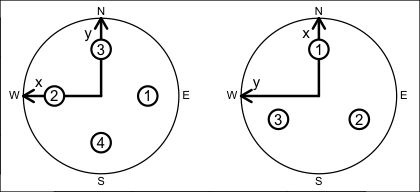
The bin geometry of a four-beam profiler is illustrated below, for adp[["beamAngle"]] equal to 20 degrees, adp[["bin1Distance"]] equal to 2m, and adp[["cellSize"]] equal to 1m. In the diagram, the viewer is in the plane containing two beams that are not shown, so the two visible beams are separated by 40 degrees. Circles indicate the centres of the range-gated bins within the beams. The lines enclosing those circles indicate the coverage of beams that spread plus and minus 2.5 degrees from their centreline.

Figure: adpgeometry2.png

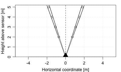
Note that adp[["oceCoordinate"]] stores the present coordinate system of the object, and it has possible values "beam", "xyz", "sfm" or "enu". (This should not be confused with adp[["originalCoordinate"]], which stores the coordinate system used in the original data file.)

The data slot holds some standardized items, and many that vary from instrument to instrument. One standard item is adp[["v"]], a three-dimensional numeric array of velocities in m/s. In this matrix, the first index indicates time, the second bin number, and the third beam number. The meaning of beams number depends on whether the object is in beam coordinates, frame coordinates, or earth coordinates. For example, if in earth coordinates, then beam 1 is the eastward component of velocity. Thus, for example,

library(oce)
data(adp)
t <- adp[["time"]]
d <- adp[["distance"]]
eastward <- adp[["v"]][,,1]
imagep(t, d, eastward, missingColor="gray")

plots an image of the eastward component of velocity as a function of time (the x axis) and distance from sensor (y axis), since the adp dataset is in earth coordinates. Note the semidurnal tidal signal, and the pattern of missing data at the ocean surface (gray blotches at the top).

Corresponding to the velocity array are two arrays of type raw, and identical dimension, accessed by adp[["a"]] and adp[["q"]], holding measures of signal strength and data quality (referred to as "correlation" in some documentation), respectively. (The exact meanings of these depend on the particular type of instrument, and it is assumed that users will be familiar enough with instruments to know both the meanings and their practical consequences in terms of data-quality assessment, etc.)

In addition to the arrays, there are time-based vectors. The vector adp[["time"]] (of length equal to the first index of adp[["v"]], etc.) holds times of observation. Depending on type of instrument and its configuration, there may also be corresponding vectors for sound speed (adp[["soundSpeed"]]), pressure (adp[["pressure"]]), temperature (adp[["temperature"]]), heading (adp[["heading"]]) pitch (adp[["pitch"]]), and roll (adp[["roll"]]), depending on the setup of the instrument.

The precise meanings of the data items depend on the instrument type. All instruments have v (for velocity), q (for a measure of data quality) and a (for a measure of backscatter amplitude, also called echo intensity). Teledyne-RDI profilers have an additional item g (for percent-good).

VmDas-equipped Teledyne-RDI profilers additional navigation data, with details listed in the table below; note that the RDI documentation (reference 2) and the RDI gui use inconsistent names for most items.

Oce name	RDI doc name	RDI GUI name
`avgSpeed`	Avg Speed	Speed/Avg/Mag
`avgMagnitudeVelocityEast`	Avg Mag Vel East	?
`avgMagnitudeVelocityNorth`	Avg Mag Vel North	?
`avgTrackMagnetic`	Avg Track Magnetic	Speed/Avg/Dir (?)
`avgTrackTrue`	Avg Track True	Speed/Avg/Dir (?)
`avgTrueVelocityEast`	Avg True Vel East	?
`avgTrueVelocityNorth`	Avg True Vel North	?
`directionMadeGood`	Direction Made Good	Speed/Made Good/Dir
`firstLatitude`	First latitude	Start Lat
`firstLongitude`	First longitude	Start Lon
`firstTime`	UTC Time of last fix	End Time
`lastLatitude`	Last latitude	End Lat
`lastLongitude`	Last longitude	End Lon
`lastTime`	UTC Time of last fix	End Time
`numberOfHeadingSamplesAveraged`	Number heading samples averaged	?
`numberOfMagneticTrackSamplesAveraged`	Number of magnetic track samples averaged	?
`numberOfPitchRollSamplesAvg`	Number of magnetic track samples averaged	?
`numberOfSpeedSamplesAveraged`	Number of speed samples averaged	?
`numberOfTrueTrackSamplesAvg`	Number of true track samples averaged	?
`primaryFlags`	Primary Flags	?
`shipHeading`	Heading	?
`shipPitch`	Pitch	?
`shipRoll`	Roll	?
`speedMadeGood`	Speed Made Good	Speed/Made Good/Mag
`speedMadeGoodEast`	Speed MG East	?
`speedMadeGoodNorth`	Speed MG North	?

For Teledyne-RDI profilers, there are four three-dimensional arrays holding beamwise data. In these, the first index indicates time, the second bin number, and the third beam number (or coordinate number, for data in xyz, sfm, enu or other coordinate systems). In the list below, the quoted phrases are quantities as defined in Figure 9 of reference 1.

v is velocity in m/s, inferred from two-byte signed integer values (multiplied by the scale factor that is stored in velocityScale in the metadata).
q is "correlation magnitude" a one-byte quantity stored as type raw in the object. The values may range from 0 to 255.
a is "backscatter amplitude", also known as "echo intensity" a one-byte quantity stored as type raw in the object. The values may range from 0 to 255.
g is "percent good" a one-byte quantity stored as raw in the object. The values may range from 0 to 100.

Finally, there is a vector adp[["distance"]] that indicates the bin distances from the sensor, measured in metres along an imaginary centre line bisecting beam pairs. The length of this vector equals dim(adp[["v"]])[2].

Teledyne-RDI Sentinel V ADCPs

As of 2016-09-27 there is provisional support for the TRDI "SentinelV" ADCPs, which are 5 beam ADCPs with a vertical centre beam. Relevant vertical beam fields are called adp[["vv"]], adp[["va"]], adp[["vq"]], and adp[["vg"]] in analogy with the standard 4-beam fields.

Accessing and altering information within adp objects

Extracting values Matrix data may be accessed as illustrated above, e.g. or an adp object named adv, the data are provided by adp[["v"]], adp[["a"]], and adp[["q"]]. As a convenience, the last two of these can be accessed as numeric (as opposed to raw) values by e.g. adp[["a", "numeric"]]. The vectors are accessed in a similar way, e.g. adp[["heading"]], etc. Quantities in the metadata slot are also available by name, e.g. adp[["velocityResolution"]], etc.

Assigning values. This follows the standard form, e.g. to increase all velocity data by 1 cm/s, use adp[["v"]] <- 0.01 + adp[["v"]].

Overview of contents The show method (e.g. show(d)) displays information about an ADP object named d.

Dealing with suspect data

There are many possibilities for confusion with adp devices, owing partly to the flexibility that manufacturers provide in the setup. Prudent users will undertake many tests before trusting the details of the data. Are mean currents in the expected direction, and of the expected magnitude, based on other observations or physical constraints? Is the phasing of currents as expected? If the signals are suspect, could an incorrect scale account for it? Could the transformation matrix be incorrect? Might the data have exceeded the maximum value, and then “wrapped around” to smaller values? Time spent on building confidence in data quality is seldom time wasted.

References

Teledyne-RDI, 2007. WorkHorse commands and output data format. P/N 957-6156-00 (November 2007).
Teledyne-RDI, 2012. VmDas User's Guide, Ver. 1.46.5.

Trim an AD2CP File

Description

Create an AD2CP file by copying the first n data chunks (regions starting with 0xa5, etc) of another such file. This can be useful in supplying small sample files for bug reports.

Usage

adpAd2cpFileTrim(infile, n = 100L, outfile, debug = getOption("oceDebug"))

Arguments

infile

name of an AD2CP file.

n

integer indicating the number of data chunks to keep. The default is to keep 100 chunks, a common choice for sample files.

outfile

optional name of the new AD2CP file to be created. If this is not supplied, a default is used, by adding ⁠_trimmed⁠ to the base filename, e.g. if infile is "a.ad2cp" then outfile will be a_trimmed.ad2cp.

debug

an integer value indicating the level of debugging. If this is 1L, then a brief indication is given of the processing steps. If it is > 1L, then information is given about each data chunk, which can yield very extensive output.

Value

adpAd2cpFileTrim() returns the name of the output file, outfile, as provided or constructed.

Sample of Usage

# Can only be run by the developer, since it uses a private file.
f  <- "~/Dropbox/oce_secret_data/ad2cp/byg_trimmed.ad2cp"
if (file.exists(f))
    adpAd2cpFileTrim(f, 100L) # this file is already trimmed to 200 chunks

Author(s)

Dan Kelley

Convert Raw to Numeric Values in an adp Object

Description

Convert variables in an adp object from raw to numeric format.

Usage

adpConvertRawToNumeric(
  object = NULL,
  variables = NULL,
  debug = getOption("oceDebug")
)

Arguments

object

an adp object.

variables

variables stored in an adp object that has the same dimensional as v and is stored in a raw format.

debug

Value

adpConvertRawToNumeric returns an adp object whose specified variables have been converted from raw to numerical format.

Author(s)

Jaimie Harbin and Dan Kelley

Examples

library(oce)
data(adp)
adp[["a"]][, , 1][, 1]
ADP <- adpConvertRawToNumeric(adp)
ADP[["a"]][, , 1][, 1]

Ensemble Average an adp Object in Time

Description

Ensemble averaging of adp objects is often necessary to reduce the uncertainty in velocity estimates from single pings. Many types of ADPs can be configured to perform the ensemble averaging during the data collection, due to memory limitations for long deployments. In cases where the instrument is not memory limited, it may be desirable to perform the ensemble averaging during post-processing, thereby reducing the overall size of the data set and decreasing the uncertainty of the velocity estimates (by averaging out Doppler noise).

Usage

adpEnsembleAverage(x, n = 5, leftover = FALSE, na.rm = TRUE, ...)

Arguments

x

an adp object.

n

number of pings to average together.

leftover

a logical value indicating how to proceed in cases where n does not divide evenly into the number of ensembles in x. If leftover is FALSE (the default) then any extra ensembles at the end of x are ignored. Otherwise, they are used to create a final ensemble in the returned value.

na.rm

a logical value indicating whether NA values should be stripped before the computation proceeds

...

extra arguments to be passed to the mean() function.

Value

A new adp object with ensembles averaged as specified. E.g. for an adp object with 100 pings and n=5 the number of rows of the data arrays will be reduced by a factor of 5.

Author(s)

Clark Richards and Dan Kelley

Examples

library(oce)
data(adp)
adpAvg <- adpEnsembleAverage(adp, n = 2)
plot(adpAvg)

Flag adp Data Past Water Column Boundary

Description

Flag variables with the same dimension of v in an adp object that are beyond the water column boundary while retaining existing flags. Currently, this operation can only be performed on adp objects that contain bottom ranges. Commonly, handleFlags() would then be used to remove such data.

Usage

adpFlagPastBoundary(
  x = NULL,
  fields = NULL,
  df = 20,
  trim = 0.15,
  good = 1,
  bad = 4,
  debug = getOption("oceDebug")
)

Arguments

x

an adp object containing bottom ranges.

fields

a variable contained within x indicating which field to flag. If NULL (the default) then adpFlagPastBoundary() applies itself to all flag fields that have the same dimensionality as v in the data slot.

df

the degrees of freedom to use during the smoothing spline operation.

trim

a scale factor for boundary trimming (see “Details”).

good

number stored in flags to indicate good data.

bad

number stored in flags to indicate bad data.

debug

Details

If the object's oceCoordinate is "beam", this works by using smooth.spline() on the time-dependent bottom ranges, beam-by-beam. If oceCoordinate is "enu", "xyz", or "other", a smooth.spline() is used on a time-dependent bottom range averaged across all the beams. The df value of the present function is passed to smooth.spline(), as a way to control smoothness. Once this is done, data within distance of 1-trim multiplied by the bottom range are flagged as being bad. The default value of trim is 0.15, which is close to the value (0.134) of 1-cos(angle*pi/180), with angle=30 as the beam angle in degrees.

Value

adpFlagPastBoundary returns an adp object with flags adjusted in the specified fields if data are beyond the water column boundary.

Author(s)

Jaimie Harbin, Clark Richards, and Dan Kelley

Trim an RDI adp File

Description

Create an RDI adp file by copying the first n data chunks (starting with byte 0x7f 0x7f) of another such file. This can be useful in supplying small sample files for bug reports.

Usage

adpRdiFileTrim(infile, n = 100L, outfile, debug = getOption("oceDebug"))

Arguments

infile

name of an RDI file.

n

integer indicating the number of data chunks to keep. The default is to keep 100 chunks, a common choice for sample files.

outfile

optional name of the new RDI file to be created. If this is not supplied, a default is used, by adding ⁠_trimmed⁠ to the base filename, e.g. if infile is "a.000" then outfile will be a_trimmed.000.

debug

an integer value indicating the level of debugging. If this is 0, then read.adp.rdi() proceeds quietly, except for issuing warnings and errors if necessary. If it is 1, then the R code of read.adp.rdi() produces some messages. If it is 2, then also the underlying C/C++ code produces a message each time a possible ensemble is detected. If it is 3, then the C/C++ code also produces information on some details of the ensemble. Levels 2 and 3 are mainly for use by the developers.

Value

adpRdiFileTrim() returns the name of the output file, outfile, as provided or constructed.

Sample of Usage

# Can only be run by the developer, since it uses a private file.
file  <- "~/data/archive/sleiwex/2008/moorings/m09/adp/rdi_2615/raw/adp_rdi_2615.000"
if (file.exists(file)) {
    adpRdiFileTrim(file, 9L, "test.000")
}

Author(s)

Dan Kelley

Sample adp File in RDI Format

Description

Sample adp File in RDI Format

Examples

read.oce(system.file("extdata", "adp_rdi.000", package="oce"))

Sample adv Data

Description

This adv object is a sampling of measurements made with a Nortek Vector acoustic Doppler velocimeter deployed as part of the St Lawrence Internal Wave Experiment (SLEIWEX). Various identifying features have been redacted.

Usage

data(adv)

Source

This file came from the SLEIWEX-2008 experiment.

Examples


library(oce)
data(adv)

# Velocity time-series
plot(adv)

# Spectrum of upward component of velocity, with ``turbulent'' reference line
s <- spectrum(adv[["v"]][, 3], plot = FALSE)
plot(log10(s$freq), log10(s$spec), type = "l")
for (a in seq(-20, 20, by = 1)) {
    abline(a = a, b = -5 / 3, col = "gray", lty = "dotted")
}

Class to Store Acoustic-Doppler Velocimeter Data

Description

This class holds data from acoustic-Doppler velocimeters.

Details

A file containing ADV data is usually recognized by Oce, and so read.oce() will usually read the data. If not, one may use the general ADV function read.adv() or specialized variants read.adv.nortek(), read.adv.sontek.adr() or read.adv.sontek.text().

ADV data may be plotted with plot,adv-method() function, which is a generic function so it may be called simply as plot(x), where x is an adv object.

Statistical summaries of ADV data are provided by the generic function summary,adv-method().

Conversion from beam to xyz coordinates may be done with beamToXyzAdv(), and from xyz to enu (east north up) may be done with xyzToEnuAdv(). toEnuAdv() may be used to transfer either beam or xyz to enu. Enu may be converted to other coordinates (e.g. aligned with a coastline) with enuToOtherAdv().

Slots

data: As with all oce objects, the data slot for adv objects is a list containing the main data for the object. The key items stored in this slot include time and v.
metadata: As with all oce objects, the metadata slot for adv objects is a list containing information about the data or about the object itself. Examples that are of common interest include frequency, oceCordinate, and frequency.
processingLog: As with all oce objects, the processingLog slot for adv objects is a list with entries describing the creation and evolution of the object. The contents are updated by various oce functions to keep a record of processing steps. Object summaries and processingLogShow() both display the log.

Modifying slot contents

Although the [[<- operator may permit modification of the contents of adv objects (see [[<-,adv-method), it is better to use oceSetData() and oceSetMetadata(), because those functions save an entry in the processingLog that describes the change.

Retrieving slot contents

The full contents of the data and metadata slots of a adv object may be retrieved in the standard R way using slot(). For example slot(o,"data") returns the data slot of an object named o, and similarly slot(o,"metadata") returns the metadata slot.

The slots may also be obtained with the [[,adv-method operator, as e.g. o[["data"]] and o[["metadata"]], respectively.

The [[,adv-method operator can also be used to retrieve items from within the data and metadata slots. For example, o[["temperature"]] can be used to retrieve temperature from an object containing that quantity. The rule is that a named quantity is sought first within the object's metadata slot, with the data slot being checked only if metadata does not contain the item. This [[ method can also be used to get certain derived quantities, if the object contains sufficient information to calculate them. For example, an object that holds (practical) salinity, temperature and pressure, along with longitude and latitude, has sufficient information to compute Absolute Salinity, and so o[["SA"]] will yield the calculated Absolute Salinity.

It is also possible to find items more directly, using oceGetData() and oceGetMetadata(), but neither of these functions can retrieve derived items.

Examples

data(adv)
adv[["v"]] <- 0.001 + adv[["v"]] # add 1mm/s to all velocity components

Trim a Sontek ADR adv File

Description

Create a Sontek ADR adv (acoustic Doppler velocimeter) file by copying the header plus the first n data chunks (recognized by the three-byte sequence 0xA5, 0x11, ‘0x3c’) into a new file. This can be useful in supplying small sample files for bug reports.

Usage

advSontekAdrFileTrim(infile, n = 100, outfile, debug = getOption("oceDebug"))

Arguments

infile

name of a Sontek ADR adp file.

n

integer indicating the number of data chunks to keep. The default is to keep 100 chunks, a common choice for sample files.

outfile

optional name of the new Sontek ADR adp file to be created. If this is not supplied, a default is used, by adding ⁠_trimmed⁠ to the base filename, e.g. if infile is "x.adr" then outfile will be x_trimmed.adr.

debug

Value

advSontekAdrFileTrim() returns the name of the output file, outfile, as provided or constructed.

Air Density

Description

Compute \rho, the in-situ density of dry air.

Usage

airRho(temperature, pressure, humidity)

Arguments

temperature

in-situ temperature, in ^\circC.

pressure

numeric value for pressure in Pa (not the kPa used in public weather forecasts).

humidity

ignored at present

Details

This will eventually be a proper equation of state, but for now it just uses a dry-air formula posted on wikipedia (i.e. not trustworthy).

Value

In-situ dry-air density, in kg/m^3.

Author(s)

Dan Kelley

References

⁠https://en.wikipedia.org/wiki/Density_of_air⁠
National Oceanographic and Atmospheric Agency, 1976. U.S. Standard Atmosphere, 1976. NOAA-S/T 76-1562. (A PDF of this document may be available at ⁠http://ntrs.nasa.gov/archive/nasa/casi.ntrs.nasa.gov/19770009539_1977009539.pdf⁠ or ⁠http://www.dtic.mil/cgi-bin/GetTRDoc?Location=U2&doc=GetTRDoc.pdf&AD=ADA035728⁠ although neither link has proven to be reliable.)

Examples

degC <- seq(0, 30, length.out = 100)
p <- seq(98, 102, length.out = 100) * 1e3
contour(x = degC, y = p, z = outer(degC, p, airRho), labcex = 1)

Sample amsr Data (Near Nova Scotia)

Description

This is a three-day composite satellite image for July 27, 2023, trimmed to show waters south and east of Nova Scotia, using code provide in the “Details” section.

Usage

data(amsr)

Details

The following code was used to create this dataset.

library(oce)
amsr <- read.amsr(download.amsr(2023, 7, 27, destdir="~/data/amsr"))
amsr <- subset(amsr, -71 < longitude & longitude < -60, debug=2)
amsr <- subset(amsr,  36 < latitude  &  latitude <  45, debug=2)

Examples

library(oce)
data(coastlineWorld)
data(amsr)
plot(amsr, "SST")
lines(coastlineWorld[["longitude"]], coastlineWorld[["latitude"]])

Class to Store AMSR-2 Satellite Data

Description

This class stores data from the AMSR-2 satellite.

Details

The Advanced Microwave Scanning Radiometer (AMSR-2) is in current operation on the Japan Aerospace Exploration Agency (JAXA) GCOM-W1 space craft, launched in May 2012. Data are processed by Remote Sensing Systems. The satellite completes an ascending and descending pass during local daytime and nighttime hours respectively. Each daily file contains 7 daytime and 7 nighttime maps of variables named as follows within the data slot of amsr objects: timeDay, SSTDay, LFwindDay (wind at 10m sensed in the 10.7GHz band), MFwindDay (wind at 10m sensed at 18.7GHz), vaporDay, cloudDay, and rainDay, along with similarly-named items that end in Night. See reference 1 for additional information on the instrument, how to cite the data source in a paper, etc.

The bands are stored in raw() form, to save storage. The accessor function [[,amsr-method can provide these values in raw form or in physical units; plot,amsr-method(), and summary,amsr-method() work with physical units.

Slots

data: As with all oce objects, the data slot for amsr objects is a list containing the main data for the object.
metadata: As with all oce objects, the metadata slot for amsr objects is a list containing information about the data or about the object itself. Examples that are of common interest include longitude and latitude, which define the grid.
processingLog: As with all oce objects, the processingLog slot for amsr objects is a list with entries describing the creation and evolution of the object. The contents are updated by various oce functions to keep a record of processing steps. Object summaries and processingLogShow() both display the log.

Modifying slot contents

Although the [[<- operator may permit modification of the contents of amsr objects (see [[<-,amsr-method), it is better to use oceSetData() and oceSetMetadata(), because those functions save an entry in the processingLog that describes the change.

Retrieving slot contents

The full contents of the data and metadata slots of a amsr object may be retrieved in the standard R way using slot(). For example slot(o,"data") returns the data slot of an object named o, and similarly slot(o,"metadata") returns the metadata slot.

The slots may also be obtained with the [[,amsr-method operator, as e.g. o[["data"]] and o[["metadata"]], respectively.

The [[,amsr-method operator can also be used to retrieve items from within the data and metadata slots. For example, o[["temperature"]] can be used to retrieve temperature from an object containing that quantity. The rule is that a named quantity is sought first within the object's metadata slot, with the data slot being checked only if metadata does not contain the item. This [[ method can also be used to get certain derived quantities, if the object contains sufficient information to calculate them. For example, an object that holds (practical) salinity, temperature and pressure, along with longitude and latitude, has sufficient information to compute Absolute Salinity, and so o[["SA"]] will yield the calculated Absolute Salinity.

It is also possible to find items more directly, using oceGetData() and oceGetMetadata(), but neither of these functions can retrieve derived items.

Author(s)

Dan Kelley and Chantelle Layton

References

Information on the satellite, how to cite the data, etc. is provided at ⁠http://www.remss.com/missions/amsr/⁠.
A simple interface for viewing and downloading data is at ⁠http://images.remss.com/amsr/amsr2_data_daily.html⁠.

Convert Astronomical Angle in Degrees to Hours, Minutes and Seconds

Description

The purpose of angle2hms is to facilitate comparison of rightAscension angles computed by sunAngle() and moonAngle() with angles reported in astronomical sources and software, which often employ an hour-minute-second notation. In that notation, decimal hour is computed as 24/360 times the angle in degrees, and from that decimal hour are compute integer hour and minute values, plus a decimal second value. It is common in the astronomical literature to use strings to represent the results, e.g. with 11^h40^m48^s.10 for the value used in the “Examples”; see Chapter 1 of Meeus (1991) for more on angle calculation and representation.

Usage

angle2hms(angle)

Arguments

angle

numerical value giving an angle in degrees

Value

angle2hms returns a list containing values time (a numerical value for decimal hour, between 0 and 24), hour, minute, and second (the last of which may have a fractional part), and string, a character value indicates the time in hour-minute-second notation, with the second part to two decimal places and intervening h, m and s characters between the units.

Author(s)

Dan Kelley

References

Meeus, Jean. Astronomical Algorithms. Second Edition. Richmond, Virginia, USA: Willmann-Bell, 1991.

Examples

# A randomly-chosen example on page 99 of Meeus (1991).
angle2hms(177.74208) # string component 11h50m58s.10

Convert Angle From 0:360 to -180:180 Convention

Description

This is mostly used for instrument heading angles, in cases where the instrument is aligned nearly northward, so that small variations in heading (e.g. due to mooring motion) can yield values that swing from small angles to large angles, because of the modulo-360 cut point. The method is to use the cosine and sine of the angle in order to find "x" and "y" values on a unit circle, and then to use atan2() to infer the angles.

Usage

angleRemap(theta)

Arguments

theta

an angle (in degrees) that is in the range from 0 to 360 degrees

Value

A vector of angles, in the range -180 to 180.

Author(s)

Dan Kelley

Examples


library(oce)
# fake some heading data that lie near due-north (0 degrees)
n <- 20
heading <- 360 + rnorm(n, sd = 10)
heading <- ifelse(heading > 360, heading - 360, heading)
x <- 1:n
plot(x, heading, ylim = c(-10, 360), type = "l", col = "lightgray", lwd = 10)
lines(x, angleRemap(heading))

Alter an Object to Account for Magnetic Declination (Generic)

Description

Current-measuring instruments that infer flow direction using magnetic compasses require a correction for magnetic declination, in order to infer currents with x and y oriented eastward and northward, respectively. applyMagneticDeclination() is a generic function that handles this task by altering velocity components (and heading values, if they exist). It works for objects of the cm, adp and adv and cm classes by calling applyMagneticDeclination,adp-method(), applyMagneticDeclination,adv-method(), or applyMagneticDeclination,cm-method(), respectively.

Usage

applyMagneticDeclination(object = "oce", declination = "ANY", debug = "ANY")

Arguments

object

an object of cm, adp, or adv class.

declination

numeric value holding magnetic declination in degrees, positive for clockwise from north.

debug

Details

The returned value is a copy of object that has been modified in 4 ways. (1) the horizontal components of velocity are rotated clockwise by declination degrees. (2) If the object holds heading values, then declination is added to them. (3) The north item in the metadata slot is set to "geographic", and a warning is issued if this was also the value in object. (4) The declination item in the metadata slot is set to the value supplied to this function.

Value

an object of the same class as object, modified as described in “Details”.

Author(s)

Dan Kelley, aided, for the adp and adv variants, by Clark Richards and Jaimie Harbin.

Alter an adp Object to Account for Magnetic Declination

Description

Acoustic-Doppler profiling instruments that infer direction using magnetic compasses to determine current direction need to have a correction applied for magnetic declination, if the goal is to infer currents with x and y oriented eastward and northward, respectively. This is what the present function does (see “Details”).

Usage

## S4 method for signature 'adp'
applyMagneticDeclination(
  object = "oce",
  declination = 0,
  debug = getOption("oceDebug")
)

Arguments

object

an adp object.

declination

numeric value holding magnetic declination in degrees, positive for clockwise from north.

debug

Details

Value

An adp object, modified as outlined in “Description”.

Author(s)

Dan Kelley, aided by Clark Richards and Jaimie Harbin.

Examples

# Transform beam coordinate to xyx, then to enu with respect to
# magnetic north, and then to geographic north.
library(oce)
file <- system.file("extdata", "adp_rdi.000", package = "oce")
lon <- -69.73433
lat <- 47.88126
beam <- read.oce(file, from = 1, to = 4, longitude = lon, latitude = lat)
dec <- magneticField(lon, lat, beam[["time"]][1])$declination
xyz <- beamToXyzAdp(beam)
# Here, we tell xyzToEnuAdp() not to set a declination,
# so enuMag has metadata$north equal to "magnetic".  We could
# also skip the use of applyMagneticDeclination() by supplying
# the known declination to xyzToEnuAdp().
enuMag <- xyzToEnuAdp(xyz, declination = NULL)
enuGeo <- applyMagneticDeclination(enuMag, declination = dec)

Alter an adv Object to Account for Magnetic Declination

Description

Acoustic-Doppler velocimetry instruments that infer direction using magnetic compasses need to have a correction applied for magnetic declination, if the goal is to infer currents with x and y oriented eastward and northward, respectively. This is what the present function does (see “Details”).

Usage

## S4 method for signature 'adv'
applyMagneticDeclination(
  object = "oce",
  declination = 0,
  debug = getOption("oceDebug")
)

Arguments

object

an adv object.

declination

numeric value holding magnetic declination in degrees, positive for clockwise from north.

debug

Details

Value

A adv object, adjusted as outlined in “Details”.

Author(s)

Dan Kelley, aided by Clark Richards and Jaimie Harbin.

Alter a cm Object to Account for Magnetic Declination

Description

Current-meter (cm) instruments determine directions from onboard compasses, so interpreting velocity components in geographical coordinates requires that magnetic declination be taken into account. This is what the present function does (see “Details”).

Usage

## S4 method for signature 'cm'
applyMagneticDeclination(
  object = "oce",
  declination = 0,
  debug = getOption("oceDebug")
)

Arguments

object

a cm object.

declination

numeric value holding magnetic declination in degrees, positive for clockwise from north.

debug

Details

Value

A cm object, adjusted as outlined in “Details”.

Author(s)

Dan Kelley

Alter an Object to Account for Magnetic Declination

Description

Usage

## S4 method for signature 'oce'
applyMagneticDeclination(
  object = "oce",
  declination = 0,
  debug = getOption("oceDebug")
)

Arguments

object

an object of cm, adp, or adv class.

declination

numeric value holding magnetic declination in degrees, positive for clockwise from north.

debug

a debugging flag, set to a positive value to get debugging.

Details

Value

an object of the same class as object, modified as outlined in “Details”.

Author(s)

Dan Kelley, aided, for the adp and adv variants, by Clark Richards and Jaimie Harbin.

Trilinear Interpolation in a 3D Array

Description

Interpolate within a 3D array, using the trilinear approximation.

Usage

approx3d(x, y, z, f, xout, yout, zout)

Arguments

x

vector of x values for grid (must be equi-spaced)

y

vector of y values for grid (must be equi-spaced)

z

vector of z values for grid (must be equi-spaced)

f

matrix of rank 3, with the gridded values mapping to the x values (first index of f), etc.

xout

vector of x values for output.

yout

vector of y values for output (length must match that of xout).

zout

vector of z values for output (length must match that of xout).

Details

Trilinear interpolation is used to interpolate within the f array, for those (xout, yout and zout) triplets that are inside the region specified by x, y and z. Triplets that lie outside the range of x, y or z result in NA values.

Value

A vector of interpolated values (or NA values), with length matching that of xout.

Author(s)

Dan Kelley and Clark Richards

Examples

# set up a grid
library(oce)
n <- 5
x <- seq(0, 1, length.out = n)
y <- seq(0, 1, length.out = n)
z <- seq(0, 1, length.out = n)
f <- array(1:n^3, dim = c(length(x), length(y), length(z)))
# interpolate along a diagonal line
m <- 100
xout <- seq(0, 1, length.out = m)
yout <- seq(0, 1, length.out = m)
zout <- seq(0, 1, length.out = m)
approx <- approx3d(x, y, z, f, xout, yout, zout)
# graph the results
plot(xout, approx, type = "l")
points(xout[1], f[1, 1, 1])
points(xout[m], f[n, n, n])

Show a Function Argument

Description

Show a Function Argument

Usage

argShow(x, nshow = 4, last = FALSE, sep = "=")

Arguments

x

the argument

nshow

number of values to show at first (if length(x)> 1)

last

indicates whether this is the final argument to the function

sep

the separator between name and value

Sample argo Data

Description

This holds data from ARGO 6900388 in the North Atlantic.

Details

Below is the official citation (note that this DOI has web links for downloads):

Argo (2017). Argo float data and metadata from Global Data Assembly Centre (Argo GDAC) - Snapshot of Argo GDAC of July, 8st 2017. SEANOE. DOI:10.17882/42182#50865

Source

The netcdf file used by read.argo() to create this argo object was downloaded using FTP to ftp.ifremer.fr/ifremer/argo/dac/bodc/6900388/6900388_prof.nc on 2020 June 24.

Examples

library(oce)
data(argo)
summary(argo)
data(coastlineWorld)
plot(argo, which = "trajectory")

Class to Store Argo Profiler Data

Description

This class stores data from Argo floats.

Details

An argo object may be read with read.argo() or created with as.argo(). Argo data can be gridded to constant pressures with argoGrid() or subsetted with subset,argo-method(). Plots can be made with plot,argo-method(), while summary,argo-method() produces statistical summaries and show produces overviews.

Slots

data: As with all oce objects, the data slot for argo objects is a list containing the main data for the object. The key items stored in this slot include equal-length vectors time, longitude, latitude and equal-dimension matrices pressure, salinity, and temperature.
metadata: As with all oce objects, the metadata slot for argo objects is a list containing information about the data or about the object itself. Examples that are of common interest include id, a vector of ID codes for the profiles, and dataMode, a vector of strings indicating whether the profile is in archived mode ("A"), realtime mode ("R"), or delayed mode ("D").
processingLog: As with all oce objects, the processingLog slot for argo objects is a list with entries describing the creation and evolution of the object. The contents are updated by various oce functions to keep a record of processing steps. Object summaries and processingLogShow() both display the log.

Modifying slot contents

Although the [[<- operator may permit modification of the contents of argo objects (see [[<-,argo-method), it is better to use oceSetData() and oceSetMetadata(), because those functions save an entry in the processingLog that describes the change.

Retrieving slot contents

The full contents of the data and metadata slots of a argo object may be retrieved in the standard R way using slot(). For example slot(o,"data") returns the data slot of an object named o, and similarly slot(o,"metadata") returns the metadata slot.

The slots may also be obtained with the [[,argo-method operator, as e.g. o[["data"]] and o[["metadata"]], respectively.

The [[,argo-method operator can also be used to retrieve items from within the data and metadata slots. For example, o[["temperature"]] can be used to retrieve temperature from an object containing that quantity. The rule is that a named quantity is sought first within the object's metadata slot, with the data slot being checked only if metadata does not contain the item. This [[ method can also be used to get certain derived quantities, if the object contains sufficient information to calculate them. For example, an object that holds (practical) salinity, temperature and pressure, along with longitude and latitude, has sufficient information to compute Absolute Salinity, and so o[["SA"]] will yield the calculated Absolute Salinity.

It is also possible to find items more directly, using oceGetData() and oceGetMetadata(), but neither of these functions can retrieve derived items.

Author(s)

Dan Kelley and Clark Richards

Grid Argo Float Data

Description

Grid an Argo float, by interpolating to fixed pressure levels. The gridding is done with approx(). If there is sufficient user demand, other methods may be added, by analogy to sectionGrid().

Usage

argoGrid(argo, p, debug = getOption("oceDebug"), ...)

Arguments

argo

A argo object to be gridded.

p

Optional indication of the pressure levels to which interpolation should be done. If this is not supplied, the pressure levels will be calculated based on the existing values, using medians. If p="levitus", then pressures will be set to be those of the Levitus atlas, given by standardDepths(), trimmed to the maximum pressure in argo. If p is a single numerical value, it is taken as the number of subdivisions to use in a call to seq() that has range from 0 to the maximum pressure in argo. Finally, if a vector numerical values is provided, then it is used as is.

debug

A flag that turns on debugging. Higher values provide deeper debugging.

...

Optional arguments to approx(), which is used to do the gridding.

Value

x an argo object.

A note about flags

Data-quality flags contained within the original object are ignored by this function, and the returned value contains no such flags. This is because such flags represent an assessment of the original data, not of quantities derived from those data. This function produces a warning to this effect. The recommended practice is to use handleFlags() or some other means to deal with flags before calling the present function.

Author(s)

Dan Kelley and Clark Richards

Examples

library(oce)
data(argo)
g <- argoGrid(argo, p = seq(0, 100, 1))
par(mfrow = c(2, 1))
t <- g[["time"]]
z <- -g[["pressure"]][, 1]
# Set zlim because of spurious temperatures.
imagep(t, z, t(g[["temperature"]]), ylim = c(-100, 0), zlim = c(0, 20))
imagep(t, z, t(g[["salinity"]]), ylim = c(-100, 0))

Convert Argo Julian Day to R Time

Description

Convert Argo Julian Day to R Time

Usage

argoJuldToTime(jday)

Arguments

jday

A numerical value indicating the julian day in the Argo convention, with day=0 at 1950-01-01.

Author(s)

Jaimie Harbin and Dan Kelley

Examples

argoJuldToTime(25749)

Convert Argo Data Name to Oce Name

Description

This function is used internally by read.argo() to convert Argo-convention data names to oce-convention names. Users should not call this directly, since its return value may be changed at any moment (e.g. to include units as well as names).

Usage

argoNames2oceNames(names, ignore.case = TRUE)

Arguments

names

vector of character strings containing names in the Argo convention.

ignore.case

a logical value passed to gsub(), indicating whether to ignore the case of input strings. The default is set to TRUE because some data files use lower-case names, despite the fact that the Argo documentation specifies upper-case.

Details

Initially, Feb 2016, the inference of names was initially done by an inspection of some data files, based on reference 1. Later, in June 2023, broader inspection of more files and documents yielded about ten additions, and a single correction: VRSpH was renamed phSensorVoltageDifference, to match related names that had been added.

It should be noted that the data files examined contain some names that are not documented in reference 1, and others that are listed only in its changelog, with no actual definitions being given. For example, the files had six distinct variable names that seem to relate to phase in the oxygen sensor, but these are not translated by the present function because these variable names are not defined in reference 1, or not defined uniquely in reference 2.

The names are converted with gsub(), using the ignore.case argument of the present function. The procedure is to first handle the items listed in the following table, with string searches anchored to the start of the string. After that, the qualifiers ⁠_ADJUSTED⁠, ⁠_ERROR⁠ and ⁠_QC⁠, are translated to Adjusted, Error, and QC, respectively.

An incomplete list of name translations is as follows, where ~ represents digit sequences in some instances and letters in others. Note that until June 2023, pHSensorVoltageDifference was called VRSpH.

Argo name	oce name
`BBP`	`bbp`
`BETA_BACKSCATTERING`	`betaBackscattering`
`BPHASE_OXY`	`bphaseOxygen`
`C~PHASE_DOXY`	`C~phaseOxygen`
`CDOM`	`CDOM`
`CNDC`	`conductivity`
`CHLA`	`chlorophyllA`
`CP`	`beamAttenuation`
`CYCLE_NUMBER`	`cycleNumber` (both this and `cycle` are handled by the [[ operator)
`DATA_CENTRE`	`dataCentre`
`DATA_MODE`	`dataMode`
`DATA_STATE_INDICATOR`	`dataStateIndicator`
`DC_REFERENCE`	`DCReference`
`DIRECTION`	`direction`
`DOWN_IRRADIANCE`	`downwellingIrradiance`
`DOWNWELLING_PAR`	`downwellingPAR`
`FIRMWARE_VERSION`	`firmwareVersion`
`FIT_ERROR_NITRATE`	`fitErrorNitrate`
`FLUORESCENCE_CDOM`	`fluorescenceCDOM`
`FLUORESCENCE_CHLA`	`fluorescenceChlorophyllA`
`IB_PH`	`pHBaseCurrent`
`IK_PH`	`pHCounterCurrent`
`INST_REFERENCE`	`instReference`
`JULD`	`juld` (and used to compute `time`)
`JULD_QC_LOCATION`	`juldQCLocation`
`LATITUDE`	`latitude`
`LONGITUDE`	`longitude`
`MOLAR_DOXY`	`oxygenUncompensated`
`MTIME`	`mtime`
`NB_SAMPLE_CTD`	`nbSampleCtd`
`PH_IN_SITU_FREE`	`pHFree`
`PH_IN_SITU_TOTAL`	`pH`
`PI_NAME`	`PIName`
`PLATFORM_NUMBER`	`id`
`POSITION_ACCURACY`	`positionAccuracy`
`POSITIONING_SYSTEM`	`positioningSystem`
`PROFILE`	`profile`
`PROJECT_NAME`	`projectName`
`RAW_DOWNWELLING_IRRADIANCE`	`rawDownwellingIrradiance`
`RAW_DOWNWELLING_PAR`	`rawDownwellingPAR`
`RAW_UPWELLING_RADIANCE`	`rawUpwellingRadiance`
`STATION_PARAMETERS`	`stationParameters`
`TEMP`	`temperature`
`TEMP_CPU_CHLA`	`temperatureCPUChlorophyllA`
`TEMP_DOXY`	`temperatureOxygen`
`TEMP_NITRATE`	`temperatureNitrate`
`TEMP_PH`	`temperaturePH`
`TEMP_SPECTROPHOTOMETER_NITRATE`	`temperatureSpectrophotometerNitrate`
`TILT`	`tilt`
`TPHASE_DOXY`	`tphaseOxygen`
`TURBIDITY`	`turbidity`
`UP_RADIANCE`	`upwellingRadiance`
`UV_INTENSITY`	`UVIntensity`
`UV_INTENSITY_DARK_NITRATE`	`UVIntensityDarkNitrate`
`UV_INTENSITY_NITRATE`	`UVIntensityNitrate`
`VRS_PH`	`pHSensorVoltageDifference`
`WMO_INST_TYPE`	`WMOInstType`

Value

A character vector of the same length as names, but with replacements having been made for all known quantities.

Author(s)

Dan Kelley, with help from Anna Victor

References

Argo User's Manual Version 3.3, Nov 89th, 2019, available at ⁠https://archimer.ifremer.fr/doc/00187/29825/⁠ online.
Argo list of parameters in an excel spreadsheet, available at ⁠http://www.argodatamgt.org/content/download/27444/187206/file/argo-parameters-list-core-and-b.xlsx⁠

Create an adp Object

Description

Create an adp Object

Usage

as.adp(
  time,
  distance,
  v,
  a = NULL,
  q = NULL,
  orientation = "upward",
  coordinate = "enu"
)

Arguments

time

of observations in POSIXct format

distance

to centre of bins

v

array of velocities, with first index for time, second for bin number, and third for beam number

a

amplitude, a raw() array with dimensions matching u

q

quality, a raw() array with dimensions matching u

orientation

a string indicating sensor orientation, e.g. "upward" and "downward"

coordinate

a string indicating the coordinate system, "enu", "beam", "xy", or "other"

Details

Construct an adp object. Only a basic subset of the typical data slot is represented in the arguments to this function, on the assumption that typical usage in reading data is to set up a nearly-blank adp object, the data slot of which is then inserted. However, in some testing situations it can be useful to set up artificial adp objects, so the other arguments may be useful.

Value

An adp object.

Author(s)

Dan Kelley

Examples

data(adp)
t <- adp[["time"]]
d <- adp[["distance"]]
v <- adp[["v"]]
a <- as.adp(time = t, distance = d, v = v)

plot(a)

Coerce Data Into an argo Object

Description

Coerce a dataset into an argo dataset. This is not the right way to read official argo datasets, which are provided in NetCDF format and may be read with read.argo().

Usage

as.argo(
  time,
  longitude,
  latitude,
  salinity,
  temperature,
  pressure,
  units = NULL,
  id,
  filename = "",
  missingValue
)

Arguments

time

a vector of POSIXct times.

longitude

a vector of longitudes.

latitude

a vector of latitudes.

salinity

a vector of salinities.

temperature

a vector of temperatures.

pressure

a vector of pressures.

units

an optional list containing units. If NULL, the default, then "degree east" is used for longitude, "degree north" for latitude, "" for salinity, "ITS-90" for temperature, and "dbar" for pressure.

id

an identifier for the argo float, typically a number, but stored within the object in a character form. (For example, the dataset retrieved with data(argo) has an id of "6900388".)

filename

a source filename, which defaults to an empty string.

missingValue

an optional missing value, indicating data values that should be taken as NA.

Value

An argo object.

Author(s)

Dan Kelley

Coerce Data Into a cm Object

Description

Coerce Data Into a cm Object

Usage

as.cm(
  time,
  u = NULL,
  v = NULL,
  pressure = NULL,
  conductivity = NULL,
  temperature = NULL,
  salinity = NULL,
  longitude = NA,
  latitude = NA,
  filename = "",
  debug = getOption("oceDebug")
)

Arguments

time

A vector of times of observation, or an oce object from which time and two velocity components can be inferred, e.g. an adv object, or an adp object that has only one distance bin. If time is an oce object, then all of the following arguments are ignored.

u, v

optional numerical vectors containing the x and y components of velocity (m/s).

pressure, conductivity, salinity, temperature

optional numerical vectors containing pressure (dbar), electrical conductivity, practical salinity, and in-situ temperature (degree C).

longitude, latitude

optional position specified in degrees East and North.

filename

optional source file name.

debug

Examples

library(oce)
# Example 1: creation from scratch
t <- Sys.time() + 0:50
u <- sin(2 * pi * 0:50 / 5) + rnorm(51)
v <- cos(2 * pi * 0:50 / 5) + rnorm(51)
p <- 100 + rnorm(51)
summary(as.cm(t, u, v, p))

# Example 2: creation from an adv object
data(adv)
summary(as.cm(adv))

Coerce Data Into a coastline Object

Description

Coerces a sequence of longitudes and latitudes into a coastline dataset. This may be used when read.coastline() cannot read a file, or when the data have been manipulated.

Usage

as.coastline(longitude, latitude, fillable = FALSE)

Arguments

longitude

the longitude in decimal degrees, positive east of Greenwich, or a data frame with columns named latitude and longitude, in which case these values are extracted from the data frame and the second argument is ignored.

latitude

the latitude in decimal degrees, positive north of the Equator.

fillable

boolean indicating whether the coastline can be drawn as a filled polygon.

Value

a coastline object.

Author(s)

Dan Kelley

Coerce Data Into a ctd Object

Description

Assemble data into a ctd object. This function is complicated (spanning approximately 500 lines of code) because it tries to handle many special cases, and tries to make sensible defaults for unspecified parameters. If odd results are found, users might find it helpful to call this function with the first argument being a simple vector of Practical Salinity values, in which case the processing of the other arguments is relatively straightforward.

Usage

as.ctd(
  salinity,
  temperature = NULL,
  pressure = NULL,
  conductivity = NULL,
  scan = NULL,
  time = NULL,
  units = NULL,
  flags = NULL,
  missingValue = NULL,
  type = "",
  serialNumber = NULL,
  ship = NULL,
  cruise = NULL,
  station = NULL,
  startTime = NULL,
  longitude = NULL,
  latitude = NULL,
  deploymentType = "unknown",
  pressureAtmospheric = 0,
  sampleInterval = NULL,
  profile = NULL,
  debug = getOption("oceDebug")
)

Arguments

salinity

may be (1) a numeric vector holding Practical Salinity, (2) a list or data frame holding salinity and other hydrographic variables or (3) an oce-class object that holds hydrographic information. If salinity is not provided, then conductivity must be provided, so that swSCTp() can be used to compute salinity.

temperature

a numeric vector containing in-situ temperature in ^\circC on the ITS-90 scale; see “Temperature units” in the documentation for swRho().

pressure

a numeric vector containing sea pressure values, in decibars. Typically, this vector has the same length as salinity and temperature, but it also possible to supply just one value, which will be repeated to get the right length. Note that as.ctd() stores the sum of pressure and pressureAtmospheric in the returned object, although the default value for pressureAtmospheric is zero, so in the default case, pressure is stored directly.

conductivity

an optional numeric vector containing electrical conductivity ratio through the water column. To convert from raw conductivity in milliSeimens per centimeter divide by 42.914 to get conductivity ratio (see Culkin and Smith, 1980).

scan

optional numeric vector holding scan number. If not provided, this is set to seq_along(salinity).

time

optional vector of times of observation.

units

an optional list containing units. If not supplied, defaults are set for pressure, temperature, salinity, and conductivity. Since these are simply guesses, users are advised strongly to supply units. See “Examples”.

flags

if supplied, this is a list containing data-quality flags. The elements of this list must have names that match the data provided to the object.

missingValue

optional missing value, indicating data that should be taken as NA. Set to NULL to turn off this feature.

type

optional type of CTD, e.g. "SBE"

serialNumber

optional serial number of instrument

ship

optional string containing the ship from which the observations were made.

cruise

optional string containing a cruise identifier.

station

optional string containing a station identifier.

startTime

optional indication of the start time for the profile, which is used in some several plotting functions. This is best given as a POSIXt time, but it may also be a character string that can be converted to a time with as.POSIXct(), using UTC as the timezone.

longitude

optional numerical value containing longitude in decimal degrees, positive in the eastern hemisphere. If this is a single number, then it is stored in the metadata slot of the returned value; if it is a vector of numbers, then they are stored in the data slot.

latitude

optional numerical value containing the latitude in decimal degrees, positive in the northern hemisphere. See the note on length, for the longitude argument.

deploymentType

character string indicating the type of deployment. Use "unknown" if this is not known, "profile" for a profile (in which the data were acquired during a downcast, while the device was lowered into the water column, perhaps also including an upcast; "moored" if the device is installed on a fixed mooring, "thermosalinograph" (or "tsg") if the device is mounted on a moving vessel, to record near-surface properties, or "towyo" if the device is repeatedly lowered and raised.

pressureAtmospheric

A numerical value (a constant or a vector), that is subtracted from pressure before storing it in the return value. (This altered pressure is also used in calculating salinity, if that is to be computed from conductivity, etc., using swSCTp(); see salinity above.)

sampleInterval

optional numerical value indicating the time between samples in the profile.

profile

optional positive integer specifying the number of the profile to extract from an object that has data in matrices, such as for some argo objects. Currently the profile argument is only utilized for argo objects.

debug

Details

The following sections provide an some notes on how as.ctd() handles certain object types given as the first parameter.

Converting argo objects

If the salinity argument is an object of argo, then that object is dismantled and reassembled as a ctd object in ways that are mostly straightforward, although the handling of time depends on the information in the original netcdf data file that was used by read.argo() to create the argo object.

All Argo data files contain an item called juld from which the profile time can be computed, and some also contain an additional item named MTIME, from which the times of individual measurements can also be computed. Both cases are handled by as.ctd(), using a scheme outlined in Note 4 of the Details section of the read.argo() documentation.

Converting rsk objects

If the salinity argument is an object of rsk, then as.ctd passes it, pressureAtmospheric, longitude, latitude ship, cruise, station and deploymentType to rsk2ctd(), which builds the ctd object that is returned by as.ctd. The other arguments to as.ctd are ignored in this instance, because rsk objects already contain their information. If required, any data or metadata element can be added to the value returned by as.ctd using oceSetData() or oceSetMetadata(), respectively.

The returned rsk object contains pressure in a form that may need to be adjusted, because rsk objects may contain either absolute pressure or sea pressure. This adjustment is handled automatically by as.ctd, by examination of the metadata item named pressureType (described in the documentation for read.rsk()). Once the sea pressure is determined, adjustments may be made with the pressureAtmospheric argument, although in that case it is better considered a pressure adjustment than the atmospheric pressure.

rsk objects may store sea pressure or absolute pressure (the sum of sea pressure and atmospheric pressure), depending on how the object was created with as.rsk() or read.rsk(). However, ctd objects store sea pressure, which is needed for plotting, calculating density, etc. This poses no difficulties, however, because as.ctd automatically converts absolute pressure to sea pressure, if the metadata in the rsk object indicates that this is appropriate. Further alteration of the pressure can be accomplished with the pressureAtmospheric argument, as noted above.

Value

A ctd object.

Author(s)

Dan Kelley

References

Culkin, F., and Norman D. Smith, 1980. Determination of the concentration of potassium chloride solution having the same electrical conductivity, at 15 C and infinite frequency, as standard seawater of salinity 35.0000 ppt (Chlorinity 19.37394 ppt). IEEE Journal of Oceanic Engineering, volume 5, pages 22-23.

Examples

library(oce)
# 1. fake data, with default units
pressure <- 1:50
temperature <- 10 - tanh((pressure - 20) / 5) + 0.02 * rnorm(50)
salinity <- 34 + 0.5 * tanh((pressure - 20) / 5) + 0.01 * rnorm(50)
ctd <- as.ctd(salinity, temperature, pressure)
# Add a new column
fluo <- 5 * exp(-pressure / 20)
ctd <- oceSetData(ctd,
    name = "fluorescence", value = fluo,
    unit = list(unit = expression(mg / m^3), scale = "")
)
summary(ctd)

# 2. fake data, with supplied units (which are the defaults, actually)
ctd <- as.ctd(salinity, temperature, pressure,
    units = list(
        salinity = list(unit = expression(), scale = "PSS-78"),
        temperature = list(unit = expression(degree * C), scale = "ITS-90"),
        pressure = list(unit = expression(dbar), scale = "")
    )
)

Coerce Data Into an echosounder Object

Description

Coerces a dataset into a echosounder dataset.

Usage

as.echosounder(
  time,
  depth,
  a,
  src = "",
  sourceLevel = 220,
  receiverSensitivity = -55.4,
  transmitPower = 0,
  pulseDuration = 400,
  beamwidthX = 6.5,
  beamwidthY = 6.5,
  frequency = 41800,
  correction = 0
)

Arguments

time

times of pings.

depth

depths of samples within pings.

a

matrix of echo amplitudes, as would be stored with read.echosounder().

src

optional string indicating data source.

sourceLevel

source level, in dB (uPa at 1m), denoted sl in reference 1 p15, where it is in units 0.1dB (uPa at 1m).

receiverSensitivity

receiver sensitivity of the main element, in dB(counts/uPa), denoted rs in reference 1 p15, where it is in units of 0.1dB(counts/uPa)

transmitPower

transmit power reduction factor, in dB, denoted tpow in reference 1 p10, where it is in units 0.1 dB.

pulseDuration

duration of transmitted pulse in us

beamwidthX

x-axis -3dB one-way beamwidth in deg, denoted bwx in reference 1 p16, where the unit is 0.2 deg

beamwidthY

y-axis -3dB one-way beamwidth in deg, denoted bwx in reference 1 p16, where the unit is 0.2 deg

frequency

transducer frequency in Hz, denoted fq in reference 1 p16

correction

user-defined calibration correction in dB, denoted corr in reference 1 p14, where the unit is 0.01dB.

Details

Creates an echosounder file. The defaults for e.g. transmitPower are taken from the echosounder dataset, and they are unlikely to make sense generally. The first three parameters must be supplied, and the dimension of a must align with the lengths of time and depths. The other parameters have defaults that are unlikely to be correct for arbitrary application, but they are not essential for basic plots, etc.

Those who use the readHAC package to read echosounder data should note that it stores the a matrix in a flipped and transposed format. See that package's demo code for a function named flip() that transforms the matrix as required by as.echosounder(). Indeed, users working with HAC data ought to study the whole of the readHAC documentation, to learn what data are stored, so that oceSetMetadata() and oceSetData() can be used as needed to flesh out the contents returned by as.echosounder().

Value

An echosounder object.

Author(s)

Dan Kelley

Coerce Data Into a gps Object

Description

Coerces a sequence of longitudes and latitudes into a GPS dataset. This may be used when read.gps() cannot read a file, or when the data have been manipulated.

Usage

as.gps(longitude, latitude, filename = "")

Arguments

longitude

latitude

the latitude in decimal degrees, positive north of the Equator.

filename

name of file containing data (if applicable).

Value

A gps object.

Author(s)

Dan Kelley

Examples

# Location of the Tower Tank at Dalhousie University
towerTank <- as.gps(-63.59428, 44.63572)

Coerce Data Into an ladp object

Description

This function assembles vectors of pressure and velocity, possibly also with shears, salinity, temperature, etc.

Usage

as.ladp(
  longitude,
  latitude,
  station,
  time,
  pressure,
  u,
  v,
  uz,
  vz,
  salinity,
  temperature,
  ...
)

Arguments

longitude

longitude in degrees east, or an oce object that contains the data otherwise given by longitude and the other arguments.

latitude

latitude in degrees east (use negative in southern hemisphere).

station

number or string indicating station ID.

time

time at the start of the profile, constructed by e.g. as.POSIXct().

pressure

pressure in decibars, through the water column.

u

eastward velocity (m/s).

v

northward velocity (m/s).

uz

vertical derivative of eastward velocity (1/s).

vz

vertical derivative of northward velocity (1/s).

salinity

salinity through the water column, in practical salinity units.

temperature

temperature through the water column.

...

optional additional data columns.

Value

An ladp object.

Author(s)

Dan Kelley

Coerce Data Into a lisst Object

Description

If data contains fewer than 42 columns, an error is reported. If it contains more than 42 columns, only the first 42 are used. This is used by read.lisst(), the documentation on which explains the meanings of the columns.

Usage

as.lisst(
  data,
  filename = "",
  year = 0,
  tz = "UTC",
  longitude = NA,
  latitude = NA
)

Arguments

data

A table (or matrix) containing 42 columns, as in a LISST data file.

filename

Name of file containing the data.

year

Year in which the first observation was made. This is necessary because LISST timestamps do not indicate the year of observation. The default value is odd enough to remind users to include this argument.

tz

Timezone of observations. This is necessary because LISST timestamps do not indicate the timezone.

longitude

Longitude of observation.

latitude

Latitude of observation.

Value

A lisst object.

Author(s)

Dan Kelley

Coerce Data Into a lobo Object

Description

Coerce a dataset into a lobo dataset.

Usage

as.lobo(
  time,
  u,
  v,
  salinity,
  temperature,
  pressure,
  nitrate,
  fluorescence,
  filename = ""
)

Arguments

time

vector of times of observation

u

vector of x velocity component observations

v

vector of y velocity component observations

salinity

vector of salinity observations

temperature

vector of temperature observations

pressure

vector of pressure observations

nitrate

vector of nitrate observations

fluorescence

vector of fluorescence observations

filename

source filename

Value

A lobo object.

Author(s)

Dan Kelley

Coerce Data Into a met Object

Description

Coerces a dataset into a met dataset. This fills in only a few of the typical data fields, so the returned object is much sparser than the output from read.met(). Also, almost no metadata fields are filled in, so the resultant object does not store station location, units of the data, data-quality flags, etc. Anyone working with data from Environment Canada (reference 2) is advised to use read.met() instead of the present function.

Usage

as.met(time, temperature, pressure, u, v, filename = "(constructed from data)")

Arguments

time

Either a vector of observation times (or character strings that can be coerced into times) or the output from canadaHCD::hcd_hourly (see reference 1).

temperature

vector of temperatures.

pressure

vector of pressures.

u

vector of eastward wind speed in m/s.

v

vector of northward wind speed in m/s.

filename

optional string indicating data source

Value

A met object.

Author(s)

Dan Kelley

References

The canadaHCD package is in development by Gavin Simpson; see ⁠https://github.com/gavinsimpson/canadaHCD⁠ for instructions on how to download and install from GitHub.
Environment Canada website for Historical Climate Data ⁠https://climate.weather.gc.ca/index_e.html⁠

Coerce Something Into an oce Object

Description

Coerce Something Into an oce Object

Usage

as.oce(x, ...)

Arguments

x

an item containing data. This may be data frame, list, or an oce object.

...

optional extra arguments, passed to conversion functions as.coastline() or ODF2oce(), if these are used.

Details

This function is limited and not intended for common use. In most circumstances, users should employ a function such as as.ctd() to construct specialized oce sub-classes.

as.oce creates an oce object from data contained within its first argument, which may be a list, a data frame, or an object of oce. (In the last case, x is simply returned, without modification.)

If x is a list containing items named longitude and latitude, then as.coastline() is called (with the specified ... value) to create a coastline object.

If x is a list created by read_odf() from the (as yet unreleased) ODF package developed by the Bedford Institute of Oceanography, then ODF2oce() is called (with no arguments other than the first) to calculate a return value. If the sub-class inference made by ODF2oce() is incorrect, users should call that function directly, specifying a value for its coerce argument.

If x has not been created by read_odf(), then the names of the items it contains are examined, and used to try to infer the proper return value. There are only a few cases (although more may be added if there is sufficient user demand). The cases are as follows.

If x contains items named temperature, pressure and either salinity or conductivity, then an object of type ctd will be returned.
If x contains columns named longitude and latitude, but no other columns, then an object of class coastline is returned.

Value

An oce object.

Coerce Data Into a rsk Object

Description

Create a rsk object.

Usage

as.rsk(
  time,
  columns,
  filename = "",
  instrumentType = "rbr",
  serialNumber = "",
  model = "",
  sampleInterval = NA,
  debug = getOption("oceDebug")
)

Arguments

time

a vector of times for the data.

columns

a list or data frame containing the measurements at the indicated times; see “Details”.

filename

optional name of file containing the data.

instrumentType

type of instrument.

serialNumber

serial number for instrument.

model

instrument model type, e.g. "RBRduo".

sampleInterval

sampling interval. If given as NA, then this is estimated as the median difference in times.

debug

a flag that can be set to TRUE to turn on debugging.

Details

The contents of columns are be copied into the data slot of the returned object directly, so it is critical that the names and units correspond to those expected by other code dealing with rsk objects. If there is a conductivity, it must be called conductivity, and it must be in units of mS/cm. If there is a temperature, it must be called temperature, and it must be an in-situ value recorded in ITS-90 units. And if there is a pressure, it must be absolute pressure (sea pressure plus atmospheric pressure) and it must be named pressure. No checks are made within as.rsk on any of these rules, but if they are broken, you may expect problems with any further processing.

Value

An rsk object.

Author(s)

Dan Kelley

Coerce Data Into a sealevel Object

Description

Coerces a dataset (minimally, a sequence of times and heights) into a sealevel dataset. The arguments are based on the standard data format, as were described in a file formerly available at reference 1.

Usage

as.sealevel(
  elevation,
  time,
  header = NULL,
  stationNumber = NA,
  stationVersion = NA,
  stationName = NULL,
  region = NULL,
  year = NA,
  longitude = NA,
  latitude = NA,
  GMTOffset = NA,
  decimationMethod = NA,
  referenceOffset = NA,
  referenceCode = NA,
  deltat
)

Arguments

elevation

a list of sea-level heights in metres, in an hourly sequence.

time

optional list of times, in POSIXct format. If missing, the list will be constructed assuming hourly samples, starting at 0000-01-01 00:00:00.

header

a character string as read from first line of a standard data file.

stationNumber

three-character string giving station number.

stationVersion

single character for version of station.

stationName

the name of station (at most 18 characters).

region

the name of the region or country of station (at most 19 characters).

year

the year of observation.

longitude

the longitude in decimal degrees, positive east of Greenwich.

latitude

the latitude in decimal degrees, positive north of the equator.

GMTOffset

offset from GMT, in hours.

decimationMethod

a coded value, with 1 meaning filtered, 2 meaning a simple average of all samples, 3 meaning spot readings, and 4 meaning some other method.

referenceOffset

referenceCode

deltat

optional interval between samples, in hours (as for the ts() timeseries function). If this is not provided, and t can be understood as a time, then the difference between the first two times is used. If this is not provided, and t cannot be understood as a time, then 1 hour is assumed.

Value

A sealevel object (for details, see read.sealevel()).

Author(s)

Dan Kelley

References

⁠http://ilikai.soest.hawaii.edu/rqds/hourly.fmt⁠ (this link worked for years but failed at least temporarily on December 4, 2016).

Examples

library(oce)

# Construct a year of M2 tide, starting at the default time
# 0000-01-01T00:00:00.
h <- seq(0, 24 * 365)
elevation <- 2.0 * sin(2 * pi * h / 12.4172)
sl <- as.sealevel(elevation)
summary(sl)

# As above, but start at the Y2K time.
time <- as.POSIXct("2000-01-01") + h * 3600
sl <- as.sealevel(elevation, time)
summary(sl)

Create a Section

Description

Create a section based on columnar data, or a set of oce objects that can be coerced to a section. There are three cases.

Usage

as.section(
  salinity,
  temperature,
  pressure,
  longitude,
  latitude,
  station,
  sectionId = "",
  debug = getOption("oceDebug")
)

Arguments

salinity

This may be a numerical vector, in which case it is interpreted as the salinity, and the other arguments are used for the other components of ctd objects. Alternatively, it may be one of a variety of other objects from which the CTD objects can be inferred, in which case the other arguments are ignored; see “Details”.

temperature

Temperature, in a vector holding values for all stations.

pressure

Pressure, in a vector holding values for all stations.

longitude

Longitude, in a vector holding values for all stations.

latitude

Latitude, in a vector holding values for all stations.

station

Station identifiers, in a vector holding values for all stations.

sectionId

Section identifier.

debug

an integer value that controls whether as.section() prints information during its work. The function works quietly if this is 0 and prints out some information if it is positive.

Details

Case 1. If the first argument is a numerical vector, then it is taken to be the salinity, and factor() is applied to station to break the data up into chunks that are assembled into ctd objects with as.ctd() and combined to make a section object to be returned. This mode of operation is provided as a convenience for datasets that are already partly processed; if original CTD data are available, the next mode is preferred, because it permits the storage of much more data and metadata in the CTD object.

Case 2. If the first argument is a list containing oce objects, then those objects are taken as profiles of something. A requirement for this to work is that every element of the list contains both longitude and latitude in either the metadata or data slot (in the latter case, the mean value is recorded in the section object) and that every element also contains pressure in its data slot.

Case 3. If the first argument is a argo object, then the profiles it contains are turned into ctd objects, and these are assembled into a section to be returned.

Value

An object of section.

Author(s)

Dan Kelley

Examples

library(oce)
data(ctd)
# vector of names of CTD objects
fake <- ctd
fake[["temperature"]] <- ctd[["temperature"]] + 0.5
fake[["salinity"]] <- ctd[["salinity"]] + 0.1
fake[["longitude"]] <- ctd[["longitude"]] + 0.01
fake[["station"]] <- "fake"
sec1 <- as.section(c("ctd", "fake"))
summary(sec1)
# vector of CTD objects
ctds <- vector("list", 2)
ctds[[1]] <- ctd
ctds[[2]] <- fake
sec2 <- as.section(ctds)
summary(sec2)
# argo data (a subset)
data(argo)
sec3 <- as.section(subset(argo, profile < 5))
summary(sec3)

Create tidem Object From Fitted Harmonic Data

Description

This function takes a set of tidal constituent amplitudes and phases, and constructs a return value of similar form to that returned by tidem(). Its purpose is to enable predictions based on published constituent amplitudes and phases. Since as.tidem() does not account for a reference height, it is the user's responsible to account for this after a prediction is made using predict.tidem().

Usage

as.tidem(
  tRef,
  latitude,
  name,
  amplitude,
  phase,
  frequency,
  speed,
  debug = getOption("oceDebug")
)

Arguments

tRef

a POSIXt value indicating the mean time of the observations used to develop the harmonic model. This is rounded to the nearest hour in as.tidem(), to match the behaviour of tidem().

latitude

numerical value indicating the latitude of the observations that were used to create the harmonic model. This is needed for nodal-correction procedures carried out by tidemVuf().

name

character vector holding names of constituents.

amplitude, phase

numeric vectors of constituent amplitudes and phases. These must be of the same length as name.

frequency, speed

optional numeric vectors giving the frequencies of the constituents (in cycles per hour) or the analogous speeds (in degrees per hour). Only one of these may be given, and a conversion is done from the latter to the former, if required. If the frequencies are thus specified, then these are used instead of the frequencies that oce normally used, as defined in data(tideconst). A warning will be issued if the absolute value of the relative frequency mismatch for any given component exceeds 1e-6, and this will occur for any NOAA tables containing the SA component, for which this relative mismatch is approximately 4e-5 (see reference 5).

debug

Details

All the constituent names used by tidem() are permitted here, except for "Z0" (see “Description” regarding reference height). To get a list of constituent names, please consult Foreman (1978), or type the following in an R console:

data(tidedata)
data.frame(name=tidedata$const$name, freq=tidedata$const$freq)

In addition to the above, as.tidem() can handle NOAA names of constituents. For the most part, these match oce names, but there are 4 exceptions: NOAA names "LAM2", "M1", "RHO", and "2MK3" are converted to oce names "LDA2", "NO1", "RHO1", and "MO3". The name mapping was inferred by matching frequencies; for these constituents, the fractional mismatch in frequencies was under 4e-8; see Reference 5 for more details. A message is printed if these name conversions are required in the particular use of as.tidem().

Apart from the standard oce names and this set of NOAA synonyms, any other constituent name is reported in a warning message.

Value

An object of tidem, with only minimal contents.

Known issues

There are two known differences between tidem() and the Matlab T_TIDE package, as listed in references 3 and 4.

References

Foreman, M. G. G., 1978. Manual for Tidal Currents Analysis and Prediction. Pacific Marine Science Report. British Columbia, Canada: Institute of Ocean Sciences, Patricia Bay.
Wikipedia, "Theory of Tides." https://en.wikipedia.org/wiki/Theory_of_tides Downloaded Aug 17, 2019.
Github issue 1653 "tidem() and t_tide do not produce identical results" (https://github.com/dankelley/oce/issues/1653)
Github issue 1654 "predict(tidem()) uses all constituents, unlike T_TIDE" (https://github.com/dankelley/oce/issues/1654)
Github issue 2143 "mismatch in oce/NOAA frequency of SA tidal constituent" (https://github.com/dankelley/oce/issues/2143)

Examples


# Example 1: show agreement with tidem()
data(sealevelTuktoyaktuk)
# 'm0' is model fitted by tidem()
m0 <- tidem(sealevelTuktoyaktuk)
p0 <- predict(m0, sealevelTuktoyaktuk[["time"]])
m1 <- as.tidem(
    mean(sealevelTuktoyaktuk[["time"]]), sealevelTuktoyaktuk[["latitude"]],
    m0[["name"]], m0[["amplitude"]], m0[["phase"]]
)
# Test agreement with tidem() result, by comparing predicted sealevels.
p1 <- predict(m1, sealevelTuktoyaktuk[["time"]])
stopifnot(max(abs(p1 - p0), na.rm = TRUE) < 1e-10)

# Example 2: See the effect of dropping weak constituents
m0[["name"]][which(m0[["amplitude"]] > 0.05)]
h <- "
name  amplitude      phase
  Z0 1.98061875   0.000000
  MM 0.21213065 263.344739
 MSF 0.15605629 133.795004
  O1 0.07641438  74.233130
  K1 0.13473817  81.093134
 OO1 0.05309911 235.749693
  N2 0.08377108  44.521462
  M2 0.49041340  77.703594
  S2 0.22023705 137.475767"
coef <- read.table(text = h, header = TRUE)
m2 <- as.tidem(
    mean(sealevelTuktoyaktuk[["time"]]),
    sealevelTuktoyaktuk[["latitude"]],
    coef$name, coef$amplitude, coef$phase
)
p2 <- predict(m2, sealevelTuktoyaktuk[["time"]])
par(mfrow = c(3, 1))
oce.plot.ts(sealevelTuktoyaktuk[["time"]], p0)
ylim <- par("usr")[3:4] # to match scales in other panels
oce.plot.ts(sealevelTuktoyaktuk[["time"]], p1, ylim = ylim)
oce.plot.ts(sealevelTuktoyaktuk[["time"]], p2, ylim = ylim)

Coerce Data Into a topo Object

Description

Coerce Data Into a topo Object

Usage

as.topo(longitude, latitude, z, filename = "")

Arguments

longitude

Either a vector of longitudes (in degrees east, and bounded by -180 and 180), or a bathy object created by getNOAA.bathy() from the marmap package; in the second case, all other arguments are ignored.

latitude

A vector of latitudes.

z

A matrix of heights (positive over land).

filename

Name of data (used when called by read.topo().

Value

A topo object.

Author(s)

Dan Kelley

Convert a String to a Unit

Description

This converts strings to unit objects. Only a few strings are recognized, because most oce functions have specialized unit vocabularies and so have little need of this function.

Usage

as.unit(u, default = list(unit = expression(), scale = ""))

Arguments

u

A character string indicating a unit. Case is ignored, so that e.g. "dbar" and "DBAR" yield equal results. The following are recognized: c("m-1", "dbar", "decibar", "degree", "degree_Celcius", "degree_north", "degree_east", "ipts-68", "its-90", "m/s^1", "m/s^2", "pss-78", "umol/kg", "micromole/kg")

default

A default to be used for the return value, if u is not a recognized string.

Value

A list with elements unit, an expression(), and scale, a string.

Author(s)

Dan Kelley

Examples

as.unit("DBAR")
as.unit("IPTS-68")
as.unit("ITS-90")
as.unit("PSS-78")
as.unit("UMOL/KG")

Create a windrose Object

Description

Create a wind-rose object, typically for plotting with plot,windrose-method().

Usage

as.windrose(x, y, dtheta = 15, debug = getOption("oceDebug"))

Arguments

x

The x component of wind speed (or stress) or an object of class met (see met), in which case the u and v components of that object are used for the components of wind speed, and y here is ignored.

y

The y component of wind speed (or stress).

dtheta

The angle increment (in degrees) within which to classify the data.

debug

A flag that turns on debugging. Set to 1 to get a moderate amount of debugging information, or to 2 to get more.

Value

A windrose object, with data slot containing

Item	Meaning
`n`	the number of `x` values
`x.mean`	the mean of the `x` values
`y.mean`	the mean of the `y` values
`theta`	the central angle (in degrees) for the class
`count`	the number of observations in this class
`mean`	the mean of the observations in this class
`fivenum`	the `fivenum()` vector for observations in this class (the min, the lower hinge, the median, the upper hinge, and the max)

Author(s)

Dan Kelley, with considerable help from Alex Deckmyn.

Examples

library(oce)
set.seed(1234)
theta <- seq(0, 360, 0.25)
x <- 1 + cos(pi / 180 * theta) + rnorm(theta)
y <- sin(pi / 180 * theta) + rnorm(theta)
wr <- as.windrose(x, y)
summary(wr)

Create an xbt Object

Description

Create an xbt Object

Usage

as.xbt(
  z,
  temperature,
  longitude = NA,
  latitude = NA,
  filename = "",
  sequenceNumber = NA,
  serialNumber = ""
)

Arguments

z

numeric vector giving vertical coordinates of measurements. This is the negative of depth, i.e. z is 0 at the air-sea interface, and negative within the water column.

temperature

numeric vector giving in-situ temperatures at the z values.

longitude, latitude

location in degE and degN.

filename

character value naming source file.

sequenceNumber

numerical value of the sequence number of the XBT drop.

serialNumber

character value holding the serial number of the XBT.

Value

An xbt object.

Author(s)

Dan Kelley

Convert a BCD Value to an Integer Value

Description

Convert a BCD Value to an Integer Value

Usage

bcdToInteger(x, endian = c("little", "big"))

Arguments

x

a raw value, or vector of raw values, coded in binary-coded decimal.

endian

character string indicating the endian-ness ("big" or "little"). The PC/intel convention is to use "little", and so most data files are in that format.

Value

An integer, or list of integers.

Author(s)

Dan Kelley

Examples

library(oce)
twenty.five <- bcdToInteger(as.raw(0x25))
thirty.seven <- as.integer(as.raw(0x25))

Get Names of Acoustic-Doppler Beams

Description

Get Names of Acoustic-Doppler Beams

Usage

beamName(x, which)

Arguments

x

an adp object.

which

an integer indicating beam number.

Value

A character string containing a reasonable name for the beam, of the form "beam 1", etc., for beam coordinates, "east", etc. for enu coordinates, "u", etc. for "xyz", or "u'", etc., for "other" coordinates. The coordinate system is determined with x[["coordinate"]].

Author(s)

Dan Kelley

Change the Coordinate System in an adv or adp Object

Description

Convert velocity data from an acoustic-Doppler velocimeter or acoustic-Doppler profiler from one coordinate system to another.

Usage

beamToXyz(x, ...)

Arguments

x

an adp or adv object.

...

extra arguments that are passed on to beamToXyzAdp() or beamToXyzAdv().

Value

An object of the same class as x, but with velocities in xyz coordinates instead of beam coordinates.

Author(s)

Dan Kelley

Convert adp Object From Beam to XYZ Coordinates

Description

Convert ADP velocity components from a beam-based coordinate system to a xyz-based coordinate system. The action depends on the type of object. Objects creating by reading RDI Teledyne, Sontek, and some Nortek instruments are handled directly.

Usage

beamToXyzAdp(x, debug = getOption("oceDebug"))

Arguments

x

an adp object.

debug

Details

For a 3-beam Nortek aquadopp object, the beams are transformed into velocities using the matrix stored in the header.

For 4-beam objects (and for the slanted 4 beams of 5-beam objects), the along-beam velocity components B_1 B_2, B_3, and B_4 are converted to Cartesian velocity components u v and w using formulae from section 5.5 of RD Instruments (1998), viz. the along-beam velocity components B_1, B_2, B_3, and B_4 are used to calculate velocity components in a cartesian system referenced to the instrument using the following formulae: u=ca(B_1-B_2), v=ca(B_4-B_3), w=-b(B_1+B_2+B_3+B_4). In addition to these, an estimate of the error in velocity is computed as e=d(B_1+B_2-B_3-B_4). The geometrical factors in these formulae are: c is +1 for convex beam geometry or -1 for concave beam geometry, a=1/(2\sin\theta) where \theta is the angle the beams make to the axial direction (which is available as x[["beamAngle"]]), b=1/(4\cos\theta), and d=a/\sqrt{2}.

Value

An object with the first 3 velocity indices having been altered to represent velocity components in xyz (or instrument) coordinates. (For rdi data, the values at the 4th velocity index are changed to represent the "error" velocity.) To indicate the change, the value of x[["oceCoordinate"]] is changed from beam to xyz.

Author(s)

Dan Kelley

References

Teledyne RD Instruments. “ADCP Coordinate Transformation: Formulas and Calculations,” January 2010. P/N 951-6079-00.
WHOI/USGS-provided Matlab code for beam-enu transformation ⁠http://woodshole.er.usgs.gov/pubs/of2005-1429/MFILES/AQDPTOOLS/beam2enu.m⁠

Convert From Beam to XYZ Coordinates (AD2CP adp Data)

Description

This looks at all the items in the data slot of x, to see if they contain an array named v that holds velocity. If that velocity has 4 components, and if oceCoordinate for the item is "beam", then along-beam velocity components B_1 B_2, B_3, and B_4 are converted to instrument-oriented Cartesian velocity components u v and w using the convex-geometry formulae from section 5.5 of reference 1, viz. u=ca(B_1-B_2), v=ca(B_4-B_3), w=-b(B_1+B_2+B_3+B_4). In addition to these, an estimate of the error in velocity is computed as e=d(B_1+B_2-B_3-B_4). The geometrical factors in these formulae are: a=1/(2\sin\theta) where \theta is the angle the beams make to the axial direction (which is available as x[["beamAngle"]]), b=1/(4\cos\theta), and d=a/\sqrt{2}.

Usage

beamToXyzAdpAD2CP(x, debug = getOption("oceDebug"))

Arguments

x

an adp object.

debug

References

Teledyne RD Instruments. “ADCP Coordinate Transformation: Formulas and Calculations,” January 2010. P/N 951-6079-00.

Convert adv Object from Beam Coordinates to XYZ Coordinates

Description

Convert ADV velocity components from a beam-based coordinate system to a xyz-based coordinate system.

Usage

beamToXyzAdv(x, debug = getOption("oceDebug"))

Arguments

x

an adv object.

debug

a flag that, if non-zero, turns on debugging. Higher values yield more extensive debugging.

Details

The coordinate transformation is done using the transformation matrix contained in transformation.matrix in the metadata slot, which is normally inferred from the header in the binary file. If there is no such matrix (e.g. if the data were streamed through a data logger that did not capture the header), beamToXyzAdv the user will need to store one in x, e.g. by doing something like the following:

x[["transformation.matrix"]] <- rbind(c(11100, -5771, -5321),
                                      c( #' 291, 9716, -10002),
                                      c( 1409, 1409, 1409)) / 4096

Author(s)

Dan Kelley

References

⁠https://nortek.zendesk.com/hc/en-us/articles/360029820971-How-is-a-Coordinate-transformation-done-⁠

Adjust adp Object to Account for Spherical Spreading

Description

Compensate ADP signal strength for spherical spreading.

Usage

beamUnspreadAdp(
  x,
  count2db = c(0.45, 0.45, 0.45, 0.45),
  asMatrix = FALSE,
  debug = getOption("oceDebug")
)

Arguments

x

an adp object.

count2db

a set of coefficients, one per beam, to convert from beam echo intensity to decibels.

asMatrix

a boolean that indicates whether to return a numeric matrix, as opposed to returning an updated object (in which the matrix is cast to a raw value).

debug

Details

First, beam echo intensity is converted from counts to decibels, by multiplying by count2db. Then, the signal decrease owing to spherical spreading is compensated for by adding the term 20\log10(r), where r is the distance from the sensor head to the water from which scattering is occurring. r is given by x[["distance"]].

Value

An adp object.

Author(s)

Dan Kelley

References

The coefficient to convert to decibels is a personal communication. The logarithmic term is explained in textbooks on acoustics, optics, etc.

Examples

library(oce)
data(adp)
plot(adp, which = 5) # beam 1 echo intensity
adp.att <- beamUnspreadAdp(adp)
plot(adp.att, which = 5) # beam 1 echo intensity
# Profiles
par(mar = c(4, 4, 1, 1))
a <- adp[["a", "numeric"]] # second arg yields matrix return value
distance <- adp[["distance"]]
plot(apply(a, 2, mean), distance, type = "l", xlim = c(0, 256))
lines(apply(a, 2, median), distance, type = "l", col = "red")
legend("topright", lwd = 1, col = c("black", "red"), legend = c("original", "attenuated"))
# Image
plot(adp.att, which = "amplitude", col = oce.colorsViridis(100))

Bilinear Interpolation Within a Grid

Description

This is used by topoInterpolate.

Usage

bilinearInterp(x, y, gx, gy, g)

Arguments

x

vector of x values at which to interpolate

y

vector of y values at which to interpolate

gx

vector of x values for the grid

gy

vector of y values for the grid

g

matrix of the grid values

Value

vector of interpolated values

Apply a Function to Vector Data

Description

The function FUN is applied to f in bins specified by xbreaks. The division of data into bins is done with cut().

Usage

binApply1D(x, f, xbreaks, FUN, include.lowest = FALSE, ...)

Arguments

x

a vector of numerical values.

f

a vector of data to which FUN will be applied.

xbreaks

optional vector holding values of x at the boundaries between bins. If this is not given, it is computed by calling pretty() with n=20 segments.

FUN

function that is applied to the f values in each x bin. This must take a single numeric vector as input, and return a single numeric value.

include.lowest

logical value indicating whether to include x values that equal xbreaks[1]. See “Details”.

...

optional arguments to pass to FUN.

Details

By default, the sub-intervals defined by the xbreaks argument are open on the left and closed on the right, to match the behaviour of cut(). An open interval does not include points on the boundary, and so any x values that exactly match the first breaks value will not be counted. To include such points in the calculation, set include.lowest to TRUE.

Value

A list with the following elements: xbreaks as used, xmids (the mid-points between those breaks) and result (the result of applying FUN to the f values in the designated bins).

Author(s)

Dan Kelley

Examples

library(oce)
# salinity profile (black) with 1-dbar bin means (red)
data(ctd)
plotProfile(ctd, "salinity")
p <- ctd[["pressure"]]
S <- ctd[["salinity"]]
pbreaks <- seq(0, max(p), 1)
binned <- binApply1D(p, S, pbreaks, mean)
lines(binned$result, binned$xmids, lwd = 2, col = rgb(1, 0, 0, 0.9))

Apply a Function to Matrix Data

Description

The function FUN is applied to f in bins specified by xbreaks and ybreaks.

Usage

binApply2D(x, y, f, xbreaks, ybreaks, FUN, include.lowest = FALSE, ...)

Arguments

x

a vector of numerical values.

y

a vector of numerical values.

f

a vector of data to which FUN will be applied.

xbreaks

values of x at the boundaries between the bins; calculated using pretty() if not supplied.

ybreaks

as xbreaks, but for y.

FUN

function that is applied to the f values in each (x,y) bin. This must take two numeric vectors as input, and return a single numeric value.

include.lowest

logical value indicating whether to include x values that equal xbreaks[1] and y values that equal ybreaks[1]. See “Details”.

...

optional arguments to pass to FUN.

Details

The division into bins is done with cut(), to which include.lowest is passed. By default, the x bins are open at the left and closed on the right, and the y bins are open at the bottom and closed at the top. However, if include.lowest is TRUE, then those boundary points are included in the calculation.

Value

A list with the following elements: xbreaks and ybreaks as used, mid-points xmids and ymids, and result, a matrix containing the result of applying FUN() to the f values in the designated bins.

Author(s)

Dan Kelley

Bin-average a Vector y, Based on x Values

Description

binAverage() works by calling binMean1D(), after computing the xbreaks parameter of the latter function as seq(xmin,xmax,xinc). Note that the return value of binAverage() uses only the xmids and result entries of the binMean1D() result.

Usage

binAverage(x, y, xmin, xmax, xinc, include.lowest = FALSE, na.rm = FALSE)

Arguments

x

a vector of numerical values.

y

a vector of numerical values.

xmin

x value at the lower limit of first bin; the minimum x will be used if this is not provided.

xmax

x value at the upper limit of last bin; the maximum x will be used if this is not provided.

xinc

width of bins, in terms of x value; 1/10th of xmax-xmin will be used if this is not provided.

include.lowest

logical value indicating whether to include y values for which the corresponding x is equal to xmin. See “Details”.

na.rm

logical value indicating whether to remove NA values before doing the computation of the average. This is passed to mean(), which does the work of the present function.

Details

By default, the sub-intervals defined by xmin, xinc and xmax arguments are open on the left and closed on the right, to match the behaviour of cut(). An open interval does not include points on the boundary, and so any x values that exactly match the first breaks value will not be counted. To include such points in the calculation, set include.lowest to TRUE.

Value

A list with two elements: x, the mid-points of the bins, and y, the average y value in the bins.

Author(s)

Dan Kelley

Examples

library(oce)
# A. fake linear data
x <- seq(0, 100, 1)
y <- 1 + 2 * x
plot(x, y, pch = 1)
ba <- binAverage(x, y)
points(ba$x, ba$y, pch = 3, col = "red", cex = 3)

# B. fake quadratic data
y <- 1 + x^2
plot(x, y, pch = 1)
ba <- binAverage(x, y)
points(ba$x, ba$y, pch = 3, col = "red", cex = 3)

# C. natural data
data(co2)
plot(co2)
avg <- binAverage(time(co2), co2, 1950, 2000, 2)
points(avg$x, avg$y, col = "red")

Bin-count Vector Data

Description

Count the number of elements of a given vector that fall within successive pairs of values within a second vector.

Usage

binCount1D(x, xbreaks, include.lowest = FALSE)

Arguments

x

vector of numerical values.

xbreaks

Vector of values of x at the boundaries between bins, calculated using pretty() if not supplied.

include.lowest

logical value indicating whether to include x values that equal xbreaks[1]. See “Details”.

Details

To contextualize binCount1D() in terms of base R functions, note that

binCount1D(1:20, seq(0, 20, 2))$number

matches

unname(table(cut(1:20, seq(0, 20, 2))))

Value

A list with the following elements: the breaks (xbreaks, midpoints (xmids) between those breaks, and the count (number) of x values between successive breaks.

Author(s)

Dan Kelley

Bin-count Matrix Data

Description

Count the number of elements of a given matrix z=z(x,y) that fall within successive pairs of breaks in x and y.

Usage

binCount2D(x, y, xbreaks, ybreaks, flatten = FALSE, include.lowest = FALSE)

Arguments

x, y

vectors of numerical values.

xbreaks, ybreaks

vector of values of x and y at the boundaries between the 2D bins, calculated using pretty() on each of x and y, if not supplied.

flatten

A logical value indicating whether the return value also contains equilength vectors x, y, z and n, a flattened representation of xmids, ymids, result and number.

include.lowest

logical value indicating whether to include points where x equals xbreaks[1] or y equals ybreaks[1].

Details

By default, the sub-intervals defined by xbreaks and ybreaks are open on the left/bottom and closed on the right/top, to match the behaviour of cut(). An open interval does not include points on the boundary, and so any x and y values that equal xbreaks[1] or ybreaks[1] will not be counted. To include such points in the calculation, set include.lowest to TRUE.

Value

A list with the following elements: the breaks (xbreaks and ybreaks), the midpoints (xmids and ymids) between those breaks, and the count (number) of f values in the boxes defined between successive breaks.

Author(s)

Dan Kelley

Bin-average f=f(x)

Description

Average the values of a vector f in bins defined on another vector x. The values are broken up into bins using cut().

Usage

binMean1D(x, f, xbreaks, include.lowest = FALSE, na.rm = FALSE)

Arguments

x

vector of numerical values that will be categorized into bins via the xbreaks parameter.

f

vector of numerical values that are associated with the x values.

xbreaks

vector of values of x at the boundaries between bins, calculated using pretty() if not supplied.

include.lowest

logical value indicating whether to include x values that equal xbreaks[1]. See “Details”.

na.rm

logical value indicating whether to remove NA values before doing the computation of the average. This is passed to mean(), which does the work of the present function.

Details

Value

A list with the following elements: the breaks (xbreaks, midpoints (xmids) between those breaks, the count (number) of x values between successive breaks, and the resultant average (result) of f, classified by the x breaks.

Author(s)

Dan Kelley

Examples

# Plot raw temperature profile as circles, with lines indicating
# the result of averaging in 1-metre depth intervals.
library(oce)
data(ctd)
z <- ctd[["z"]]
T <- ctd[["temperature"]]
plot(T, z, cex = 0.3)
TT <- binMean1D(z, T, seq(-100, 0, 1))
lines(TT$result, TT$xmids, col = rgb(1, 0, 0, 0.9), lwd = 2)

Bin-average f=f(x,y)

Description

Average the values of a vector f(x,y) in bins defined on vectors x and y. A common example might be averaging spatial data into location bins.

Usage

binMean2D(
  x,
  y,
  f,
  xbreaks,
  ybreaks,
  flatten = FALSE,
  fill = FALSE,
  fillgap = -1,
  include.lowest = FALSE,
  na.rm = FALSE,
  debug = getOption("oceDebug")
)

Arguments

x

vector of numerical values.

y

vector of numerical values.

f

Matrix of numerical values, a matrix f=f(x,y).

xbreaks

Vector of values of x at the boundaries between bins, calculated using pretty(x) if not supplied.

ybreaks

Vector of values of y at the boundaries between bins, calculated using pretty(y) if not supplied.

flatten

a logical value indicating whether the return value also contains equilength vectors x, y, z and n, a flattened representation of xmids, ymids, result and number.

fill, fillgap

values controlling whether to attempt to fill gaps (that is, regions of NA values) in the matrix. If fill is false, gaps, or regions with NA values, are not altered. If fill is TRUE, then gaps that are of size less than or equal to fillgap are interpolated across, by calling fillGapMatrix() with the supplied value of fillgap.

include.lowest

logical value indicating whether to include y values for which the corresponding x is equal to xmin. See “Details”.

na.rm

logical value indicating whether to remove NA values before doing the computation of the average. This is passed to mean(), which does the work of the present function.

debug

Value

By default, i.e. with flatten being FALSE, binMean2D() returns a list with the following elements: xmids, a vector holding the x-bin midpoints; ymids, a vector holding the y-bin midpoints; number, a matrix holding the number the points in each bin; and result, a matrix holding the mean value in each bin. If flatten is TRUE, the number and result matrices are renamed as n and f and transformed to vectors, while the bin midpoints are renamed as x and y and extended to match the length of n and f.

Author(s)

Dan Kelley

Examples

library(oce)
x <- runif(500, 0, 0.5)
y <- runif(500, 0, 0.5)
f <- x^2 + y^2
xb <- seq(0, 0.5, 0.1)
yb <- seq(0, 0.5, 0.1)
m <- binMean2D(x, y, f, xb, yb)
cm <- colormap(f, col = oceColorsTurbo)
opar <- par(no.readonly = TRUE)
drawPalette(colormap = cm)
plot(x, y, col = cm$zcol, pch = 20, cex = 1.4)
contour(m$xmids, m$ymids, m$result, add = TRUE, labcex = 1.4)
par(opar)

Bin-map an adp Object

Description

Bin-map an ADP object, by interpolating velocities, backscatter amplitudes, etc., to uniform depth bins, thus compensating for the pitch and roll of the instrument. This only makes sense for ADP objects that are in beam coordinates.

Usage

binmapAdp(x, debug = getOption("oceDebug"))

Arguments

x

an adp object.

debug

Value

An adp object.

Bugs

This only works for 4-beam RDI ADP objects.

Sample of Usage

library(oce)
file <- "~/data/archive/sleiwex/2008/moorings/m09/adp/rdi_2615/raw/adp_rdi_2615.000"
beam <- read.oce(file,
    from=as.POSIXct("2008-06-26", tz="UTC"),
    to=as.POSIXct("2008-06-26 00:10:00", tz="UTC"),
    longitude=-69.73433, latitude=47.88126)
beam2 <- binmapAdp(beam)
plot(enuToOther(toEnu(beam), heading=-31.5))
plot(enuToOther(toEnu(beam2), heading=-31.5))
plot(beam, which=5:8) # backscatter amplitude
plot(beam2, which=5:8)

Author(s)

Dan Kelley and Clark Richards

References

The method was devised by Clark Richards for use in his PhD work at Department of Oceanography at Dalhousie University.

Calculate a Bound, Rounded up to Mantissa 1, 2, or 5

Description

Calculate a Bound, Rounded up to Mantissa 1, 2, or 5

Usage

bound125(x)

Arguments

x

a single positive number

Value

for positive x, a value exceeding x that has mantissa 1, 2, or 5; otherwise, x

Class to Store Bremen-formatted Data

Description

This class is for data stored in a format used at Bremen. It is somewhat similar to the odf, in the sense that it does not apply just to a particular instrument. Although some functions are provided for dealing with these data (see “Details”), the most common action is to read the data with read.bremen(), and then to coerce the object to another storage class (e.g. using as.ctd() for CTD-style data) so that specialized functions can be used thereafter.

Slots

data: As with all oce objects, the data slot for bremen objects is a list containing the main data for the object.
metadata: As with all oce objects, the metadata slot for bremen objects is a list containing information about the data or about the object itself.
processingLog: As with all oce objects, the processingLog slot for bremen objects is a list with entries describing the creation and evolution of the object. The contents are updated by various oce functions to keep a record of processing steps. Object summaries and processingLogShow() both display the log.

Modifying slot contents

Although the [[<- operator may permit modification of the contents of bremen objects (see [[<-,bremen-method), it is better to use oceSetData() and oceSetMetadata(), because those functions save an entry in the processingLog that describes the change.

Retrieving slot contents

The full contents of the data and metadata slots of a bremen object may be retrieved in the standard R way using slot(). For example slot(o,"data") returns the data slot of an object named o, and similarly slot(o,"metadata") returns the metadata slot.

The slots may also be obtained with the [[,bremen-method operator, as e.g. o[["data"]] and o[["metadata"]], respectively.

The [[,bremen-method operator can also be used to retrieve items from within the data and metadata slots. For example, o[["temperature"]] can be used to retrieve temperature from an object containing that quantity. The rule is that a named quantity is sought first within the object's metadata slot, with the data slot being checked only if metadata does not contain the item. This [[ method can also be used to get certain derived quantities, if the object contains sufficient information to calculate them. For example, an object that holds (practical) salinity, temperature and pressure, along with longitude and latitude, has sufficient information to compute Absolute Salinity, and so o[["SA"]] will yield the calculated Absolute Salinity.

It is also possible to find items more directly, using oceGetData() and oceGetMetadata(), but neither of these functions can retrieve derived items.

Author(s)

Dan Kelley

Format Bytes as Binary (Defunct)

Description

WARNING: The endian argument will soon be removed from this function; see oce-defunct. This is because the actions for endian="little" made no sense in practical work. The default value for endian was changed to "big" on 2017 May 6.

Usage

byteToBinary(x, endian = "big")

Arguments

x

an integer to be interpreted as a byte.

endian

character string indicating the endian-ness ("big" or "little"). WARNING: This argument will be removed soon.

Value

A character string representing the bit strings for the elements of x, in order of significance for the endian="big" case. (The nibbles, or 4-bit sequences, are interchanged in the now-deprecated "little" case.) See “Examples” for how this relates to the output from rawToBits.

Author(s)

Dan Kelley

Examples

library(oce)
# Note comparison with rawToBits():
a <- as.raw(0x0a)
byteToBinary(a, "big") # "00001010"
as.integer(rev(rawToBits(a))) # 0 0 0 0 1 0 1 0

Sample cm Data

Description

The result of using read.cm() on a current meter file holding measurements made with an Interocean S4 device. See read.cm() for some general cautionary notes on reading such files. Note that the salinities in this sample dataset are known to be incorrect, perhaps owing to a lack of calibration of an old instrument that had not been used in a long time.

Usage

data(cm)

Examples

library(oce)
data(cm)
summary(cm)
plot(cm)

Class to Store Current Meter Data

Description

This class stores current meter data, e.g. from an Interocean/S4 device or an Aanderaa/RCM device.

Slots

data: As with all oce objects, the data slot for cm objects is a list containing the main data for the object. The key items stored in this slot are time, u and v.
metadata: As with all oce objects, the metadata slot for cm objects is a list containing information about the data or about the object itself.
processingLog: As with all oce objects, the processingLog slot for cm objects is a list with entries describing the creation and evolution of the object. The contents are updated by various oce functions to keep a record of processing steps. Object summaries and processingLogShow() both display the log.

Modifying slot contents

Although the [[<- operator may permit modification of the contents of cm objects (see [[<-,cm-method), it is better to use oceSetData() and oceSetMetadata(), because those functions save an entry in the processingLog that describes the change.

Retrieving slot contents

The full contents of the data and metadata slots of a cm object may be retrieved in the standard R way using slot(). For example slot(o,"data") returns the data slot of an object named o, and similarly slot(o,"metadata") returns the metadata slot.

The slots may also be obtained with the [[,cm-method operator, as e.g. o[["data"]] and o[["metadata"]], respectively.

The [[,cm-method operator can also be used to retrieve items from within the data and metadata slots. For example, o[["temperature"]] can be used to retrieve temperature from an object containing that quantity. The rule is that a named quantity is sought first within the object's metadata slot, with the data slot being checked only if metadata does not contain the item. This [[ method can also be used to get certain derived quantities, if the object contains sufficient information to calculate them. For example, an object that holds (practical) salinity, temperature and pressure, along with longitude and latitude, has sufficient information to compute Absolute Salinity, and so o[["SA"]] will yield the calculated Absolute Salinity.

It is also possible to find items more directly, using oceGetData() and oceGetMetadata(), but neither of these functions can retrieve derived items.

Author(s)

Dan Kelley

Infer Variable Name, Units and Scale From a Seabird Header

Description

This function is used by read.ctd.sbe() to infer data names and units from the coding used by Teledyne/Seabird (SBE) .cnv files. Lacking access to documentation on the SBE format, the present function is based on inspection of a suite of CNV files available to the oce developers.

Usage

cnvName2oceName(h, columns = NULL, debug = getOption("oceDebug"))

Arguments

h

The header line.

columns

Optional list containing name correspondences, as described for read.ctd.sbe().

debug

Details

A few sample header lines that have been encountered are:

# name 4 = t068: temperature, IPTS-68 [deg C]
# name 3 = t090C: Temperature [ITS-90, deg C]
# name 4 = t190C: Temperature, 2 [ITS-90, deg C]

Examination of several CNV files suggests that it is best to try to infer the name from the characters between the "=" and ":" characters, because the material after the colon seems to vary more between sample files.

The table given below indicates the translation patterns used. These are taken from reference 1. The .cnv convention for multiple sensors is to include optional extra digits in the name, and these are indicated with ~ or ⁠~~⁠ in the table; their decoding is done with grep().

It is important to note that this table is by no means complete, since there are a great many SBE names listed in their document (reference 1), plus names not listed there but present in data files supplied by prominent archiving agencies. If an SBE name is not recognized, then the oce name is set to that SBE name. This can cause problems in some other processing steps (e.g. if swRho() or a similar function is called with an oce object as first argument), and so users are well-advised to rename the items as appropriate. The first step in doing this is to pass the object to summary(), to discover the SBE names in question. Then consult the SBE documentation to find an appropriate name for the data, and either manipulate the names in the object data slot directly or use oceRenameData() to rename the elements. Finally, please publish an 'issue' on the oce Github site ⁠https://github.com/dankelley/oce/issues⁠ so that the developers can add the data type in question. (To save development time, there is no plan to add all possible data types without a reasonable and specific expression user interest. Oxygen alone has over forty variants.)

Key	Result	Unit;scale	Notes
`accM`	`acceleration`	m/s^2
`altM`	`altimeter`	m
`alt`	`altimeter`	m
`⁠bat~⁠`	`beamAttenuation`	1/m
`C2-C1mS/cm`	`conductivityDifference`	mS/cm
`C2-C1S/m`	`conductivityDifference`	S/m
`C2-C1uS/cm`	`conductivityDifference`	uS/cm
`cond~mS/cm`	`conductivity`	mS/cm
`cond~S/m`	`conductivity`	S/m
`cond~uS/cm`	`conductivity`	uS/cm
`⁠CStarAt~⁠`	`beamAttenuation`	1/m
`⁠CStarTr~⁠`	`beamTransmission`	percent
`c~mS/cm`	`conductivity`	mS/cm
`c~S/m`	`conductivity`	S/m
`c~uS/cm`	`conductivity`	uS/cm
`⁠density~~⁠`	`density`	kg/m^3
`depFM`	`depth`	m
`depF`	`depth`	m
`depSM`	`depth`	m
`depS`	`depth`	m
`dz/dtM`	`descentRate`	m/s
`flCM`	`fluorescence`	ug/l; Chelsea Mini Chl Con
`⁠flCUVA~⁠`	`fluorescence`	ug/l; Chelsea UV Aquatracka
`⁠flC~⁠`	`fluorescence`	ug/l; Chelsea Aqua 3
`⁠flEC-AFL~⁠`	`fluorescence`	mg/m^3; WET Labs ECO-AFL/FLtab
`⁠flScufa~⁠`	`fluorescence`	-; Turner SCUFA (RFU)
`flSPR`	`fluorescence`	-; Seapoint, Rhodamine
`flSPuv`	`fluorescence`	-; Seapoint, UV
`flSP`	`fluorescence`	-; Seapoint
`flS`	`fluorescence`	-; Seatech
`flT`	`fluorescence`	-; Turner 10-005 flT
`⁠f~⁠`	`frequency`	Hz
`⁠f~~⁠`	`frequency`	Hz
`gpa`	`geopotentialAnomaly`	-; J/kg
`latitude`	`latitude`	degN
`longitude`	`longitude`	degE
`n2satMg/L`	`nitrogenSaturation`	mg/l
`n2satML/L`	`nitrogenSaturation`	ml/l
`n2satumol/kg`	`nitrogenSaturation`	umol/kg
`nbin`	`nbin`
`⁠obsscufa~⁠`	`backscatter`	NTU; Turner SCUFA
`opoxMg/L`	`oxygen`	mg/l; Optode, Aanderaa
`opoxML/L`	`oxygen`	ml/l; Optode, Aanderaa
`opoxMm/L`	`oxygen`	umol/l; Optode, Aanderaa
`opoxPS`	`oxygen`	percent; Optode, Aanderaa
`oxsatMg/L`	`oxygen`	mg/l; Weiss
`oxsatML/L`	`oxygen`	ml/l; Weiss
`oxsatMm/Kg`	`oxygen`	umol/kg; Weiss
`oxsolMg/L`	`oxygen`	mg/l; Garcia-Gordon
`oxsolML/L`	`oxygen`	ml/l; Garcia-Gordon
`oxsolMm/Kg`	`oxygen`	umol/kg; Garcia-Gordon
`par/log`	`PAR`	log; Satlantic
`⁠par~⁠`	`PAR`	-; Biospherical/Licor
`ph`	`pH`	-
`⁠potemp~68C⁠`	`thetaM`	degC; IPTS-68
`⁠potemp~90C⁠`	`thetaM`	degC; ITS-90
`pr50M`	`pressure`	dbar; SBE50
`prDE`	`pressure`	psi; digiquartz	2
`prdE`	`pressure`	psi; strain gauge	2
`prDM`	`pressure`	dbar; digiquartz
`prdM`	`pressure`	dbar; strain gauge
`prM`	`pressure`	dbar
`prSM`	`pressure`	dbar
`prSM`	`pressure`	dbar; strain gauge
`pr`	`pressure`	dbar	1
`ptempC`	`pressureTemperature`	degC; ITS-90	3
`pumps`	`pumpStatus`
`⁠rhodflTC~⁠`	`Rhodamine`	ppb; Turner Cyclops
`⁠sal~~⁠`	`salinity`	-, PSS-78	4
`sbeox~ML/L`	`oxygen`	ml/l; SBE43
`sbeox~Mm/Kg`	`oxygen`	umol/kg; SBE43
`sbeox~Mm/L`	`oxygen`	umol/l; SBE43
`sbeox~PS`	`oxygen`	percent; SBE43
`sbeox~V`	`oxygenRaw`	V; SBE43
`sbox~dV/dT`	`oxygen`	dov/dt; SBE43
`sbox~ML/L`	`oxygen`	ml/l; SBE43
`sbox~Mm/Kg`	`oxygen`	umol/kg; SBE43
`sbox~Mm/L`	`oxygen`	umol/l; SBE43
`sbox~PS`	`oxygen`	percent; SBE43
`sbox~V`	`oxygenRaw`	V; SBE43
`scan`	`scan`	-
`⁠seaTurbMtr~⁠`	`turbidity`	FTU; Seapoint
`secS-priS`	`salinityDifference`	-, PSS-78
`sigma-`é	`sigmaTheta`	kg/m^3	5
`sigma-t`	`sigmaT`	kg/m^3
`sigma-theta`	`sigmaTheta`	kg/m^3	5
`spar`	`spar`	-
`specc`	`specificConductance`	uS/cm
`sva`	`specificVolumeAnomaly`	1e-8 m^3/kg;
`⁠svCM~⁠`	`soundSpeed`	m/s; Chen-Millero
`t090Cm`	`temperature`	degC; ITS-90
`t190C`	`temperature`	degC; ITS-90
`⁠T2~68C⁠`	`temperatureDifference`	degC; IPTS-68
`⁠T2~90C⁠`	`temperatureDifference`	degC; ITS-90
`⁠t3868C~⁠`	`temperature`	degC; IPTS-68
`⁠t3890C~⁠`	`temperature`	degC; ITS-90
`⁠t38~38C⁠`	`temperature`	degC; IPTS-68
`⁠t38~90C⁠`	`temperature`	degC; ITS-90
`t4968C`	`temperature`	degC; IPTS-68
`t4990C`	`temperature`	degC; ITS-90
`timeH`	`timeH`	hour; elapsed
`timeJV2`	`timeJV2`	julian day
`timeJ`	`timeJ`	julian day
`timeK`	`timeK`	s; since Jan 1, 2000
`timeM`	`timeM`	minute; elapsed
`timeN`	`timeN`	s; NMEA since Jan 1, 1970
`timeQ`	`timeQ`	s; NMEA since Jan 1, 2000
`timeS`	`timeS`	s; elapsed
`tnc268C`	`temperature`	degC; IPTS-68
`tnc290C`	`temperature`	degC; ITS-90
`tnc68C`	`temperature`	degC; IPTS-68
`tnc90C`	`temperature`	degC; ITS-90
`tsa`	`thermostericAnomaly`	1e-8 m^3/kg
`turbflTCdiff`	`turbidityDifference`	NTU; Turner Cyclops
`⁠turbflTC~⁠`	`turbidity`	NTU; Turner Cyclops
`turbWETbbdiff`	`turbidityDifference`	1/(m\*sr); WET Labs ECO
`⁠turbWETbb~⁠`	`turbidity`	1/(m\*sr); WET Labs ECO
`turbWETntudiff`	`turbidityDifference`	NTU; WET Labs ECO
`⁠turbWETntu~⁠`	`turbidity`	NTU; WET Labs ECO
`tv268C`	`temperature`	degC; IPTS-68
`tv290C`	`temperature`	degC; ITS-90
`⁠t~68C⁠`	`temperature`	degC; IPTS-68
`t~68`	`temperature`	degC; IPTS-68
`⁠t~90C⁠`	`temperature`	degC; ITS-90
`t~90`	`temperature`	degC; ITS-90
`⁠upoly~⁠`	`upoly`	-
`⁠user~⁠`	`user`	-
`⁠v~~⁠`	`voltage`	V
`wetBAttn`	`beamAttenuation`	1/m; WET Labs AC3
`wetBTrans`	`beamTransmission`	percent; WET Labs AC3
`wetCDOMdiff`	`fluorescenceDifference`	mg/m^3; WET Labs CDOM
`⁠wetCDOM~⁠`	`fluorescence`	mg/m^3; WET Labs CDOM
`wetChAbs`	`fluorescence`	1/m; WET Labs AC3 absorption
`wetStardiff`	`fluorescenceDifference`	mg/m^3; WET Labs WETstar
`⁠wetStar~⁠`	`fluorescence`	mg/m^3; WET Labs WETstar
`xmiss`	`beamTransmission`	percent; Chelsea/Seatech
`⁠xmiss~⁠`	`beamTransmission`	percent; Chelsea/Seatech

Notes:

'pr' is in a Dalhousie-generated data file but seems not to be in reference 1.
This is an odd unit, and so if ⁠sw*⁠ functions are called on an object containing this, a conversion will be made before performing the computation. Be on the lookout for errors, since this is a rare situation.
Assume ITS-90 temperature scale, since sample .cnv file headers do not specify it.
Some files have PSU for this. Should we handle that? And are there other S scales to consider?
The 'theta' symbol (here shown accented e) may appear in different ways with different encoding configurations, set up within R or in the operating system.

Author(s)

Dan Kelley

References

A SBE data processing manual was once at ⁠http://www.seabird.com/document/sbe-data-processing-manual⁠, but as of summer 2018, this no longer seems to be provided by SeaBird. A web search will turn up copies of the manual that have been put online by various research groups and data-archiving agencies. As of 2018-07-05, the latest version was named SBEDataProcessing_7.26.4.pdf and had release date 12/08/2017, and this was the reference version used in coding oce.

Class to Store Coastline Data

Description

This class stores coastline data.

Slots

data: As with all oce objects, the data slot for coastline objects is a list containing the main data for the object. The key items stored in this slot are longitude and latitude.
metadata: As with all oce objects, the metadata slot for coastline objects is a list containing information about the data or about the object itself.
processingLog: As with all oce objects, the processingLog slot for coastline objects is a list with entries describing the creation and evolution of the object. The contents are updated by various oce functions to keep a record of processing steps. Object summaries and processingLogShow() both display the log.

Modifying slot contents

Although the [[<- operator may permit modification of the contents of coastline objects (see [[<-,coastline-method), it is better to use oceSetData() and oceSetMetadata(), because those functions save an entry in the processingLog that describes the change.

Retrieving slot contents

The full contents of the data and metadata slots of a coastline object may be retrieved in the standard R way using slot(). For example slot(o,"data") returns the data slot of an object named o, and similarly slot(o,"metadata") returns the metadata slot.

The slots may also be obtained with the [[,coastline-method operator, as e.g. o[["data"]] and o[["metadata"]], respectively.

The [[,coastline-method operator can also be used to retrieve items from within the data and metadata slots. For example, o[["temperature"]] can be used to retrieve temperature from an object containing that quantity. The rule is that a named quantity is sought first within the object's metadata slot, with the data slot being checked only if metadata does not contain the item. This [[ method can also be used to get certain derived quantities, if the object contains sufficient information to calculate them. For example, an object that holds (practical) salinity, temperature and pressure, along with longitude and latitude, has sufficient information to compute Absolute Salinity, and so o[["SA"]] will yield the calculated Absolute Salinity.

It is also possible to find items more directly, using oceGetData() and oceGetMetadata(), but neither of these functions can retrieve derived items.

Author(s)

Dan Kelley

Find the Name of the Best Coastline Object

Description

Find the name of the most appropriate coastline for a given locale Checks coastlineWorld, coastlineWorldFine and coastlineWorldCoarse, in that order, to find the one most appropriate for the locale.

Usage

coastlineBest(lonRange, latRange, span, debug = getOption("oceDebug"))

Arguments

lonRange

range of longitude for locale

latRange

range of latitude for locale

span

span of domain in km (if provided, previous two arguments are ignored).

debug

set to a positive value to get debugging information during processing.

Value

The name of a coastline that can be loaded with data().

Author(s)

Dan Kelley

Cut a Coastline Object at Specified Longitude

Description

This can be helpful in preventing mapPlot() from producing ugly horizontal lines in world maps. These lines occur when a coastline segment is intersected by longitude lon_0+180. Since the coastline files in the oce and ocedata packages are already "cut" at longitudes of -180 and 180, the present function is not needed for default maps, which have +lon_0=0. However, may help with other values of lon_0.

Usage

coastlineCut(coastline, lon_0 = 0)

Arguments

coastline

a coastline object.

lon_0

longitude as would be given in a ⁠+lon_0=⁠ item in a call to sf::sf_project().

Value

a new coastline object

Caution

This function is provisional. Its behaviour, name and very existence may change. Part of the development plan is to see if there is common ground between this and the clipPolys function in the PBSmapping package.

Author(s)

Dan Kelley

Examples


library(oce)
data(coastlineWorld)
mapPlot(coastlineCut(coastlineWorld, lon_0 = 100),
    projection = "+proj=moll +lon_0=100", col = "gray"
)

Sample coastline Data (Global, at 1:110M scale)

Description

This is a coarse resolution coastline at scale 1:110M, with 10,696 points, suitable for world-scale plots plotted at a small size, e.g. inset diagrams. Finer resolution coastline files are provided in the ocedata package.

Installing your own datasets

Follow the procedure along the lines described in “Details”, where of course your source file will differ. Also, you should change the name of the coastline object from coastlineWorld, to avoid conflicts with the built-in dataset. Save the .rda file to some directory of your choosing, e.g. perhaps ⁠/data/coastlines⁠ or ⁠~/data/coastlines⁠ on a unix-type machine. Then, whenever you need the file, use load() to load it. Most users find it convenient to do the loading in an Rprofile() startup file.

Source

Downloaded from ⁠https://www.naturalearthdata.com⁠, in ne_110m_admin_0_countries.shp in July 2015, with an update on December 16, 2017.

Calculate a Color Map

Description

Create a mapping between numeric values and colors, for use in palettes and plots. The return value can be used in various ways, including colorizing points on scattergraphs, controlling images created by image() or imagep(), drawing palettes with drawPalette(), etc.

Usage

colormap(
  z = NULL,
  zlim,
  zclip = FALSE,
  breaks,
  col = oceColorsViridis,
  name,
  x0,
  x1,
  col0,
  col1,
  blend = 0,
  missingColor,
  debug = getOption("oceDebug")
)

Arguments

z

an optional vector or other set of numerical values to be examined. If z is given, the return value will contain an item named zcol that will be a vector of the same length as z, containing a color for each point. If z is not given, zcol will contain just one item, the color "black".

zlim

optional vector containing two numbers that specify the z limits for the color scale. This can only be provided in cases A and B, as defined in “Details”. For case A, if zlim is not provided, then it is inferred by using rangeExtended() on breaks, if that is provided, or from z otherwise. Also, in case A, it is an error to provide both zlim and breaks, unless the latter is of length 1, meaning the number of subdivisions to use within the range set by zlim. In case B, zlim is inferred from using rangeExtended() on c(x0,x1). In case C, providing zlim yields an error message, because it makes no sense in the context of a named, predefined color scheme.

zclip

logical, with TRUE indicating that z values outside the range of zlim or breaks should be painted with missingColor and FALSE indicating that these values should be painted with the nearest in-range color.

breaks

an optional indication of break points between color levels (see image()). If this is provided, the arguments name through blend are all ignored (see “Details”). If it is provided, then it may either be a vector of break points, or a single number indicating the desired number of break points to be computed with pretty⁠(z,breaks)⁠. In either case of non-missing breaks, the resultant break points must number 1 plus the number of colors (see col).

col

either a vector of colors or a function taking a numerical value as its single argument and returning a vector of colors. Prior to 2021-02-08, the default for col was oceColorsJet, but it was switched to oceColorsViridis on that date. The value of col is ignored if name is provided, or if x0 through col1 are provided.

name

an optional string naming a built-in colormap (one of "gmt_relief", "gmt_ocean", "gmt_globe" or "gmt_gebco") or the name of a file or URL that contains a color map specification in GMT format. If name is given, then it is passed to colormapGMT(), which creates the colormap. Note that the colormap thus created has a fixed relationship between value and color, and zlim, only other argument that is examined is z (which may be used so that zcol will be defined in the return value), and warnings are issued if some irrelevant arguments are provided.

x0, x1, col0, col1

Vectors that specify a color map. They must all be the same length, with x0 and x1 being numerical values, and col0 and col1 being colors. The colors may be strings (e.g. "red") or colors as defined by rgb() or hsv().

blend

a number indicating how to blend colors within each band. This is ignored except when x0 through col1 are supplied. A value of 0 means to use col0[i] through the interval x0[i] to x1[i]. A value of 1 means to use col1[i] in that interval. A value between 0 and 1 means to blend between the two colors according to the stated fraction. Values exceeding 1 are an error at present, but there is a plan to use this to indicate sub-intervals, so a smooth palette can be created from a few colors.

missingColor

color to use for missing values. This cannot be provided if name is also provided (case C), because named schemes have pre-defined colors. For other cases, missingColor defaults to "gray", if it is not provided as an argument.

debug

a flag that turns on debugging. Set to 1 to get a moderate amount of debugging information, or to 2 to get more.

Details

colormap can be used in a variety of ways, including the following.

Case A. Supply some combination of arguments that is sufficient to define a mapping of value to color, without providing x0, col0, x1 or col1 (see case B for these), or providing name (see Case C). There are several ways to do this. One approach is to supply z but no other argument, in which case zlim, and breaks will be determined from z, and the default col will be used. Another approach is to specify breaks and col together, in the same way as they might be specified for the base R function image(). It is also possible to supply only zlim, in which case breaks is inferred from that value. The figure below explains the ('breaks', 'col') method of specifying a color mapping. Note that there must be one more break than color. This is the method used by e.g. [image()].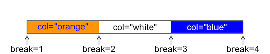
Case B. Supply x0, col0, x1, and col1, but not zlim, breaks, col or name. The x0, col0, x1 and col1 values specify a value-color mapping that is similar to that used for GMT color maps. The method works by using seq() to interpolate between the elements of the x0 vector. The same is done for x1. Similarly, colorRampPalette() is used to interpolate between the colors in the col0 vector, and the same is done for col1. The figure above explains the ('x0', 'x1', 'col0', 'col1') method of specifying a color mapping. Note that the each of the items has the same length. The case of 'blend=0', which has color 'col0[i]' between 'x0[i]' and 'x1[i]', is illustrated below.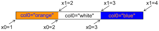
Case C. Supply name and possibly also z, but not zlim, breaks, col, x0, col0, x1 or col1. The name may be the name of a pre-defined color palette ("gmt_relief", "gmt_ocean", "gmt_globe" or "gmt_gebco"), or it may be the name of a file (or URL pointing to a file) that contains a color map in the GMT format (see “References”). If z is supplied along with name, then zcol will be set up in the return value, e.g. for use in colorizing points. Another method for finding colors for data points is to use the colfunction() function in the return value.

Value

a list containing the following (not necessarily in this order)

zcol, a vector of colors for z, if z was provided, otherwise "black"
zlim, a two-element vector suitable as the argument of the same name supplied to image() or imagep()
breaks and col, vectors of breakpoints and colors, suitable as the same-named arguments to image() or imagep()
zclip the provided value of zclip.
x0 and x1, numerical vectors of the sides of color intervals, and col0 and col1, vectors of corresponding colors. The meaning is the same as on input. The purpose of returning these four vectors is to permit users to alter color mapping, as in example 3 in “Examples”.
missingColor, a color that could be used to specify missing values, e.g. as the same-named argument to imagep().
colfunction, a univariate function that returns a vector of colors, given a vector of z values; see Example 6.

Sample of Usage

# Example 2. topographic image with a standard color scheme
par(mfrow=c(1,1))
data(topoWorld)
cm <- colormap(name="gmt_globe")
imagep(topoWorld, breaks=cm$breaks, col=cm$col)

# Example 3. topographic image with modified colors,
# black for depths below 4km.
cm <- colormap(name="gmt_globe")
deep <- cm$x0 < -4000
cm$col0[deep] <- "black"
cm$col1[deep] <- "black"
cm <- colormap(x0=cm$x0, x1=cm$x1, col0=cm$col0, col1=cm$col1)
imagep(topoWorld, breaks=cm$breaks, col=cm$col)

# Example 4. image of world topography with water colorized
# smoothly from violet at 8km depth to blue
# at 4km depth, then blending in 0.5km increments
# to white at the coast, with tan for land.
cm <- colormap(x0=c(-8000, -4000,   0,  100),
     x1=c(-4000,     0, 100, 5000),
     col0=c("violet","blue","white","tan"),
     col1=c("blue","white","tan","yellow"))
lon <- topoWorld[["longitude"]]
lat <- topoWorld[["latitude"]]
z <- topoWorld[["z"]]
imagep(lon, lat, z, breaks=cm$breaks, col=cm$col)
contour(lon, lat, z, levels=0, add=TRUE)

# Example 5. visualize GMT style color map
cm <- colormap(name="gmt_globe", debug=4)
plot(seq_along(cm$x0), cm$x0, pch=21, bg=cm$col0)
grid()
points(seq_along(cm$x1), cm$x1, pch=21, bg=cm$col1)

# Example 6. colfunction
cm <- colormap(c(0, 1))
x <- 1:10
y <- (x - 5.5)^2
z <- seq(0, 1, length.out=length(x))
drawPalette(colormap=cm)
plot(x, y, pch=21, bg=cm$colfunction(z), cex=3)

Author(s)

Dan Kelley

References

The following references provide information on choosing colour schemes, that are suitable for viewers who have colour deficiencies.

Light, Adam, and Patrick J. Bartlein. "The End of the Rainbow? Color Schemes for Improved Data Graphics." Eos, Transactions American Geophysical Union 85, no. 40 (2004): 385. DOI: 10.1029/2004EO400002

Stephenson, David B. "Comment on 'Color Schemes for Improved Data Graphics', by A Light and P.J. Bartlein." Eos, Transactions American Geophysical Union 86, no. 20 (2005): 196. DOI: 10.1029/2005EO200005

Light, Adam, and Patrick J. Bartlein. "Reply to 'Comment on Color Schemes for Improved Data Graphics,' by A. Light and P.J. Bartlein'." Eos, Transactions American Geophysical Union 86, no. 20 (2005): 196–196. DOI: 10.1029/2005EO200006

Examples

library(oce)
# Example 1. color scheme for points on xy plot
x <- seq(0, 1, length.out = 40)
y <- sin(2 * pi * x)
par(mar = c(3, 3, 1, 1))
mar <- par("mar") # prevent margin creep by drawPalette()
# First, default breaks
c <- colormap(y)
drawPalette(c$zlim, col = c$col, breaks = c$breaks)
plot(x, y, bg = c$zcol, pch = 21, cex = 1)
grid()
par(mar = mar)
# Second, 100 breaks, yielding a smoother palette
c <- colormap(y, breaks = 100)
drawPalette(c$zlim, col = c$col, breaks = c$breaks)
plot(x, y, bg = c$zcol, pch = 21, cex = 1)
grid()
par(mar = mar)

Create a GMT-type (CPT) Colormap

Description

colormapGMT creates colormaps in the Generic Mapping Tools (GMT) scheme (see References 1 to 4). A few such schemes are built-in, and may be referred to by name ("gmt_gebco", "gmt_globe", "gmt_ocean", or "gmt_relief") while others are handled by reading local files that are in GMT format, or URLs providing such files (see Reference 3).

Usage

colormapGMT(name, debug = getOption("oceDebug"))

Arguments

name

character value specifying the GMT scheme, or a source for such a scheme. Four pre-defined schemes are available, accessed by setting name to "gmt_gebco", "gmt_globe", "gmt_ocean", or "gmt_relief". If name is not one of these values, then it is taken to be the name of a local file in GMT format or, if no such file is found, a URL holding such a file.

debug

integer that, if positive, indicates to print some debugging output

Details

The GMT files understood by colormapGMT are what GMT calls "Regular CPT files" (see reference 4). This is a text format that can be read and (with care) edited in a text editor. There are three categories of lines within this file. (1) Any line starting with the "#" character is a comment, and is ignored by colormapGMT. (2) Lines with 8 numbers specify colour bands. The first number is a z value, and the three numbers after that are red, green and blue values in the range from 0 to 255. This set of 4 numbers is followed on the same line with similar values. Think of this sequence as describing a band of colours between two z values. (3) Lines starting with a character, followed by three numbers, specify particular codings. The character "B" specifies background colour, while "F" specifies foreground colour, and "N" specifies the colour to be used for missing data (the letter stands for not-a-number). Only "N" is used by colormapGMT, and it takes on the role that the missingColor argument would otherwise have. (This is why missingColor is not permitted if name is given.)

Value

colormap returns a list, in the same format as the return value for colormap().

Author(s)

Dan Kelley

References

General overview of GMT system ⁠https://www.generic-mapping-tools.org⁠.
Information on GMT color schemes ⁠https://docs.generic-mapping-tools.org/dev/cookbook/cpts.html⁠
Source of GMT specification files ⁠https://beamreach.org/maps/gmt/share/cpt/⁠
CPT (color palette table) format ⁠https://www.soest.hawaii.edu/gmt/gmt/html/GMT_Docs.html#x1-820004.15⁠

Create a Composite Object by Averaging Across Good Data

Description

Items within the data slots of the objects that are supplied as arguments are averaged in a way that makes sense for the object class, i.e. taking into account the particular bad-data codes of that particular class.

Usage

composite(object, ...)

Arguments

object

either a list of oce objects, in which case this is the only argument, or a single oce object, in which case at least one other argument (an object of the same size) must be supplied.

...

Ignored, if object is a list. Otherwise, one or more oce objects of the same sub-class as the first argument.

Create a Composite of amsr Satellite Data

Description

Form averages for each item in the data slot of the supplied objects, taking into account the bad-data codes.

Usage

## S4 method for signature 'amsr'
composite(object, ...)

Arguments

object

An amsr object.

...

Other amsr objects.

Details

If none of the objects has good data at any particular pixel (i.e. particular latitude and longitude), the resultant will have the bad-data code of the last item in the argument list. The metadata in the result are taken directly from the metadata of the final argument, except that the filename is set to a comma-separated list of the component filenames.

Composite by Averaging Across Data

Description

This is done by calling a specialized version of the function defined in the given class. In the present version, the objects must inherit from amsr, so the action is to call composite,amsr-method().

Usage

## S4 method for signature 'list'
composite(object)

Arguments

object

a list of oce objects.

Determine Available Derived Water Properties

Description

This determines what things can be derived from the supplied variables. For example, if salinity, temperature, and pressure are supplied, then potential temperature, sound speed, and several other things can be derived. If, in addition, longitude and latitude are supplied, then Absolute Salinity, Conservative Temperature, and some other things can be derived. Similarly, nitrate can be computed from NO2+NO3 together with nitrate, and nitrite can be computed from NO2+NO3 together with nitrate. See the “Examples” for a full listing.

Usage

computableWaterProperties(x)

Arguments

x

a specification of the names of known variables. This may be (a) an oce object, in which case the names are determined by calling names() on the data slot of x, or (b) a vector of character values indicating the names.

Value

computableWaterProperties() returns a sorted character vector holding the names of computable water properties, or NULL, if there are no computable values.

Author(s)

Dan Kelley

Examples

library(oce)
# Example 1
data(ctd)
computableWaterProperties(ctd)
# Example 2: nothing an be computed from just salinity
computableWaterProperties("salinity")
# Example 3: quite a lot can be computed from this trio of values
computableWaterProperties(c("salinity", "temperature", "pressure"))
# Example 4: now we can get TEOS-10 values as well
computableWaterProperties(c(
    "salinity", "temperature", "pressure",
    "longitude", "latitude"
))

Concatenate oce Objects (Generic)

Description

Concatenate oce Objects (Generic)

Usage

concatenate(object, ..., debug = getOption("oceDebug"))

Arguments

object

an oce object.

...

optional additional oce objects.

debug

integer indicating a debugging level. If this is 0, the work is done silently. If it is a larger integer, some information may be printed during the processing.

Value

An object of class corresponding to that of object.

Concatenate adp Objects

Description

This function concatenates adp objects. It is intended for objects holding data sampled through time, and it works by pasting together data linearly if they are vectors, by row if they are matrices, and by second index if they are arrays. It has been tested for the following classes: adp, adv, ctd, and met. It may do useful things for other classes, and so users are encouraged to try, and to report problems to the developers. It is unlikely that the function will do anything even remotely useful for image and topographic data, to name just two cases that do not fit the sampled-over-time category.

Usage

## S4 method for signature 'adp'
concatenate(object, ..., debug = getOption("oceDebug"))

Arguments

object

An object of adp, or a list containing such objects (in which case the remaining arguments are ignored).

...

optional additional objects of adp.

debug

integer indicating debugging level. If this exceeds 1, some information may be printed during the processing.

Value

An object of adp.

Author(s)

Dan Kelley

Examples

## 1. Split, then recombine, a ctd object.
data(ctd)
ctd1 <- subset(ctd, scan <= median(ctd[["scan"]]))
ctd2 <- subset(ctd, scan > median(ctd[["scan"]]))
CTD <- concatenate(ctd1, ctd2)

## 2. Split, then recombine, an adp object.
data(adp)
midtime <- median(adp[["time"]])
adp1 <- subset(adp, time <= midtime)
adp2 <- subset(adp, time > midtime)
ADP <- concatenate(adp1, adp2)

## Not run: 
## 3. Download two met files and combine them.
met1 <- read.met(download.met(id=6358, year=2003, month=8))
met2 <- read.met(download.met(id=6358, year=2003, month=9))
MET <- concatenate(met1, met2)

## End(Not run)

Concatenate a List of oce Objects

Description

Concatenate a List of oce Objects

Usage

## S4 method for signature 'list'
concatenate(object)

Arguments

object

a list of oce objects.

Value

An object of class corresponding to that in object.

Concatenate oce Objects (oce-Specific)

Description

This function concatenates oce objects. It is intended for objects holding data sampled through time, and it works by pasting together data linearly if they are vectors, by row if they are matrices, and by second index if they are arrays. It has been tested for the following classes: adp, adv, ctd, and met. It may do useful things for other classes, and so users are encouraged to try, and to report problems to the developers. It is unlikely that the function will do anything even remotely useful for image and topographic data, to name just two cases that do not fit the sampled-over-time category.

Usage

## S4 method for signature 'oce'
concatenate(object, ..., debug = getOption("oceDebug"))

Arguments

object

An object of oce, or a list containing such objects (in which case the remaining arguments are ignored).

...

optional additional objects of oce.

debug

integer indicating debugging level. If this exceeds 1, some information may be printed during the processing.

Value

An object of oce.

Author(s)

Dan Kelley

Examples

## 1. Split, then recombine, a ctd object.
data(ctd)
ctd1 <- subset(ctd, scan <= median(ctd[["scan"]]))
ctd2 <- subset(ctd, scan > median(ctd[["scan"]]))
CTD <- concatenate(ctd1, ctd2)

## 2. Split, then recombine, an adp object.
data(adp)
midtime <- median(adp[["time"]])
adp1 <- subset(adp, time <= midtime)
adp2 <- subset(adp, time > midtime)
ADP <- concatenate(adp1, adp2)

## Not run: 
## 3. Download two met files and combine them.
met1 <- read.met(download.met(id=6358, year=2003, month=8))
met2 <- read.met(download.met(id=6358, year=2003, month=9))
MET <- concatenate(met1, met2)

## End(Not run)

Coriolis Parameter on the Earth

Description

Compute f, the Coriolis parameter as a function of latitude (see reference 1), assuming earth siderial angular rotation rate omega=7292115e-11 rad/s. See reference 1 for general notes, and see reference 2 for comments on temporal variations of omega.

Usage

coriolis(latitude, degrees = TRUE)

Arguments

latitude

Vector of latitudes in ^\circN or radians north of the equator.

degrees

Flag indicating whether degrees are used for latitude; if set to FALSE, radians are used.

Value

Coriolis parameter, in radian/s.

Author(s)

Dan Kelley

References

Gill, A.E., 1982. Atmosphere-ocean Dynamics, Academic Press, New York, 662 pp.
Groten, E., 2004: Fundamental Parameters and Current, 2004. Best Estimates of the Parameters of Common Relevance to Astronomy, Geodesy, and Geodynamics. Journal of Geodesy, 77:724-797. (downloaded from ⁠http://www.iag-aig.org/attach/e354a3264d1e420ea0a9920fe762f2a0/51-groten.pdf⁠ March 11, 2017).

Examples

C <- coriolis(45) # 1e-4

Sample ctd Data

Description

This is a CTD profile measured in Halifax Harbour in 2003, based on ctdRaw(), but trimmed to just the downcast with ctdTrim(), using indices inferred by inspection of the results from plotScan().

Usage

data(ctd)

Details

This station was sampled by students enrolled in the Dan Kelley's Physical Oceanography class at Dalhousie University. The data were acquired near the centre of the Bedford Basin of the Halifax Harbour, during an October 2003 field trip of Dalhousie University's Oceanography 4120/5120 class. Note that the startTime in the metadata slot was altered from 1903 to 2003, using oceEdit(). The change was done because the original time was clearly incorrect, perhaps owing to the use of software that was designed to work in the twentieth century only.

Sample of Usage

library(oce)
data(ctd)
plot(ctd)

Class to Store CTD (or general hydrographic) Data

Description

This class stores hydrographic data such as measured with a CTD (conductivity, temperature, depth) instrument, or with other systems that produce similar data. Data repositories may store conductivity, temperature and depth, as in the instrument name, but it is also common to store salinity, temperature and pressure instead (or in addition). For this reason, ctd objects are required to hold salinity, temperature and pressure in their data slot, with other data being optional. Formulae are available for converting between variants of these data triplets, e.g. swSCTp() can calculate salinity given conductivity, temperature and pressure, and these are used by the main functions that create ctd objects. For example, if read.ctd.sbe() is used to read a Seabird file that contains only conductivity, temperature and pressure, then that function will automatically append a data item to hold salinity. Since as.ctd() does the same with salinity, the result this is that all ctd objects hold salinity, temperature and pressure, which are henceforth called the three basic quantities.

Details

Different units and scales are permitted for the three basic quantities, and most oce functions check those units and scales before doing calculations (e.g. of seawater density), because those calculations demand certain units and scales. The way this is handled is that the accessor function [[,ctd-method] returns values in standardized form. For example, a ctd object might hold temperature defined on the IPTS-68 scale, but e.g. ctd[["temperature"]] returns a value on the ITS-90 scale. (The conversion is done with T90fromT68().) Similarly, pressure may be stored in either dbars or PSI, but e.g. ctd[["pressure"]] returns a value in dbars, after dividing by 0.689476 if the value is stored in PSI. Luckily, there is (as of early 2016) only one salinity scale in common use in data files, namely PSS-78.

Slots

data: As with all oce objects, the data slot for ctd objects is a list containing the main data for the object. The key items stored in this slot are: salinity, temperature, and pressure, although in many instances there are quite a few additional items.
metadata: As with all oce objects, the metadata slot for ctd objects is a list containing information about the data or about the object itself. An example of the former might be the location at which a ctd measurement was made, stored in longitude and latitude, and of the latter might be filename, the name of the data source.
processingLog: As with all oce objects, the processingLog slot for ctd objects is a list with entries describing the creation and evolution of the object. The contents are updated by various oce functions to keep a record of processing steps. Object summaries and processingLogShow() both display the log.

Modifying slot contents

Although the [[<- operator may permit modification of the contents of ctd objects (see [[<-,ctd-method), it is better to use oceSetData() and oceSetMetadata(), because those functions save an entry in the processingLog that describes the change.

Retrieving slot contents

The full contents of the data and metadata slots of a ctd object may be retrieved in the standard R way using slot(). For example slot(o,"data") returns the data slot of an object named o, and similarly slot(o,"metadata") returns the metadata slot.

The slots may also be obtained with the [[,ctd-method operator, as e.g. o[["data"]] and o[["metadata"]], respectively.

The [[,ctd-method operator can also be used to retrieve items from within the data and metadata slots. For example, o[["temperature"]] can be used to retrieve temperature from an object containing that quantity. The rule is that a named quantity is sought first within the object's metadata slot, with the data slot being checked only if metadata does not contain the item. This [[ method can also be used to get certain derived quantities, if the object contains sufficient information to calculate them. For example, an object that holds (practical) salinity, temperature and pressure, along with longitude and latitude, has sufficient information to compute Absolute Salinity, and so o[["SA"]] will yield the calculated Absolute Salinity.

It is also possible to find items more directly, using oceGetData() and oceGetMetadata(), but neither of these functions can retrieve derived items.

Reading/creating `ctd` objects

A file containing CTD profile data may be read with read.ctd(), and a CTD object can also be created with as.ctd(). See read.ctd() for references on data formats used in CTD files. Data can also be assembled into ctd objects with as.ctd().

Statistical summaries are provided by summary,ctd-method(), while show() displays an overview.

CTD objects may be plotted with plot,ctd-method(), which does much of its work by calling plotProfile() or plotTS(), both of which can also be called by the user, to get fine control over the plots.

A CTD profile can be isolated from a larger record with ctdTrim(), a task made easier when plotScan() is used to examine the results. Towyow data can be split up into sets of profiles (ascending or descending) with ctdFindProfiles(). CTD data may be smoothed and/or cast onto specified pressure levels with ctdDecimate().

As with all oce objects, low-level manipulation may be done with oceSetData() and oceSetMetadata(). Additionally, many of the contents of CTD objects may be altered with the [[<-,ctd-method scheme, and sufficiently skilled users may even manipulate the contents directly.

Data sources

Archived CTD (and other) data may be found on servers such as

⁠https://cchdo.ucsd.edu/⁠

Author(s)

Dan Kelley

Examples


# 1. Create a ctd object with fake data.
a <- as.ctd(salinity = 35 + 1:3 / 10, temperature = 10 - 1:3 / 10, pressure = 1:3)
summary(a)

# 2. Fix a typo in a station latitude (fake! it's actually okay)
data(ctd)
ctd <- oceSetMetadata(
    ctd, "latitude", ctd[["latitude"]] - 0.001,
    "fix latitude typo in log book"
)

Sample ctd File in .cnv Format

Description

Sample ctd File in .cnv Format

Examples

read.oce(system.file("extdata", "ctd.cnv.gz", package="oce"))

Decimate a ctd Profile

Description

Interpolate a CTD profile to specified pressure values. This is used by sectionGrid(), but is also useful for dealing with individual CTD/bottle profiles.

Usage

ctdDecimate(
  x,
  p = 1,
  method = "boxcar",
  rule = 1,
  e = 1.5,
  na.rm = FALSE,
  debug = getOption("oceDebug")
)

Arguments

x

a ctd object.

p

pressure increment, or vector of pressures. In the first case, pressures from 0dbar to the rounded maximum pressure are used, incrementing by p dbars. If a vector of pressures is given, interpolation is done to these pressures.

method

the method to be used for calculating decimated values. This may be a string specifying the method, or a function. In the string case, the possibilities are as follows.

"boxcar" (based on a local average)
"approx" (based on linear interpolation between neighboring points, using approx() with the rule argument specified here)
"approxML" as "approx", except that a mixed layer is assumed to apply above the top data value; this is done by setting the yleft argument to approx(), and by calling that function with ⁠rule=c(2, 1))⁠
"lm" (based on local regression, with e setting the size of the local region);
"rr" for the Reiniger and Ross method, carried out with oce.approx();
"unesco" (for the UNESCO method, carried out with oce.approx().

On the other hand, if method is a function, then it must take two arguments, named data and parameters. The first is set to x@data by ctdTrim(). The second is passed directly to the user's function (see Example 2). The return value from the function must be a logical vector of the same length as the pressure data, with TRUE values meaning to keep the corresponding entries of the data slot.

rule

an integer that is passed to approx(), in the case where method is "approx". Note that the default value for rule is 1, which will inhibit extrapolation beyond the observed pressure range. This is a change from the behaviour previous to May 8, 2017, when a rule of 2 was used (without stating so as an argument).

e

is an expansion coefficient used to calculate the local neighbourhoods for the "boxcar" and "lm" methods. If e=1, then the neighbourhood for the i-th pressure extends from the (i-1)-th pressure to the (i+1)-th pressure. At the endpoints it is assumed that the outside bin is of the same pressure range as the first inside bin. For other values of e, the neighbourhood is expanded linearly in each direction. If the "lm" method produces warnings about "prediction from a rank-deficient fit", a larger value of "e" should be used.

na.rm

logical value indicating whether to remove NA values before decimating. This value is ignored unless method is boxcar in which case it is passed to binMean1D() which does the averaging. This parameter was added in February 2024, and the behaviour of ctdDecimate() prior that date was equivalent to na.rm=FALSE, so that is the default value, even though it is expected that many uses will find using TRUE is more convenient. See ⁠https://github.com/dankelley/oce/issues/2192⁠ for more discussion.

debug

Details

The "approx" and "approxML" methods may be best for bottle data, in which the usual task is to interpolate from a coarse sampling grid to a finer one. The distinction is that "approxML" assumes a mixed-layer above the top sample value. For CTD data, the "boxcar" method may be the preferred choice, because the task is normally to sub-sample, and some degree of smoothing is usually desired. (The "lm" method can be quite slow, and its results may be quite similar to those of the boxcar method.)

For widely-spaced data, a sort of numerical cabeling effect can result when density is computed based on interpolated salinity and temperature. See reference 2 for a discussion of this issue and possible solutions.

Value

A ctd object, with pressures that are as set by the "p" parameter and all other properties modified appropriately.

A note about flags

Author(s)

Dan Kelley

References

R.F. Reiniger and C.K. Ross, 1968. A method of interpolation with application to oceanographic data. Deep Sea Research, 15, 185-193.
Oguma, Sachiko, Toru Suzuki, Yutaka Nagata, Hidetoshi Watanabe, Hatsuyo Yamaguchi, and Kimio Hanawa. “Interpolation Scheme for Standard Depth Data Applicable for Areas with a Complex Hydrographical Structure.” Journal of Atmospheric and Oceanic Technology 21, no. 4 (April 1, 2004): 704-15.

Examples

library(oce)
data(ctd)
plotProfile(ctd, "salinity", ylim = c(10, 0))
p <- seq(0, 45, 1)
ctd2 <- ctdDecimate(ctd, p = p)
lines(ctd2[["salinity"]], ctd2[["pressure"]], col = "blue")
p <- seq(0, 45, 1)
ctd3 <- ctdDecimate(ctd, p = p, method = function(x, y, xout) {
    predict(smooth.spline(x, y, df = 30), xout)$y
})
lines(ctd3[["salinity"]], ctd3[["pressure"]], col = "red")

Find Profiles Within a Tow-Yow ctd Record

Description

Examine the pressure record looking for extended periods of either ascent or descent, and return either indices to these events or a vector of CTD records containing the events.

Usage

ctdFindProfiles(
  x,
  cutoff = 0.5,
  minLength = 10,
  minHeight,
  smoother = smooth.spline,
  direction = c("descending", "ascending"),
  breaks,
  arr.ind = FALSE,
  distinct,
  debug = getOption("oceDebug"),
  ...
)

Arguments

x

a ctd object.

cutoff

criterion on pressure difference; see “Details”. If not provided, this defaults to 0.5.

minLength

lower limit on number of points in candidate profiles. If not provided, this defaults to 10.

minHeight

lower limit on height of candidate profiles. If not provided, this defaults to 0.1 times the pressure span.

smoother

The smoothing function to use for identifying down/up casts. The default is smooth.spline, which performs well for a small number of cycles; see “Examples” for a method that is better for a long tow-yo. The return value from smoother must be either a list containing an element named y or something that can be coerced to a vector with as.vector(). To turn smoothing off, so that cycles in pressure are determined by simple first difference, set smoother to NULL.

direction

String indicating the travel direction to be selected.

breaks

optional integer vector indicating the indices of last datum in each profile stored within x. Thus, the first profile in the return value will contain the x data from indices 1 to breaks[1]. If breaks is given, then all other arguments except x are ignored. Using breaks is handy in cases where other schemes fail, or when the author has independent knowledge of how the profiles are strung together in x.

arr.ind

logical value indicating whether the array indices should be returned; the alternative is to return a vector of ctd objects.

distinct

An optional string indicating how to identify profiles by unique values. Use "location" to find profiles by a change in longitude and latitude, or use the name of any of item in the data slot in x. In these cases, all the other arguments except x are ignored. However, if distinct is not supplied, the other arguments are handled as described above.

debug

...

Optional extra arguments that are passed to the smoothing function, smoother.

Details

The method works by examining the pressure record. First, this is smoothed using smoother() (see “Arguments”), and then the result is first-differenced using diff(). Median values of the positive and negative first-difference values are then multiplied by cutoff. This establishes criteria for any given point to be in an ascending profile, a descending profile, or a non-profile. Contiguous regions are then found, and those that have fewer than minLength points are discarded. Then, those that have pressure ranges less than minHeight are discarded.

Caution: this method is not well-suited to all datasets. For example, the default value of smoother is smooth.spline(), and this works well for just a few profiles, but poorly for a tow-yo with a long sequence of profiles; in the latter case, it can be preferable to use simpler smoothers (see “Examples”). Also, depending on the sampling protocol, it is often necessary to pass the resultant profiles through ctdTrim(), to remove artifacts such as an equilibration phase, etc. Generally, one is well-advised to use the present function for a quick look at the data, relying on e.g. plotScan() to identify profiles visually, for a final product.

Value

If arr.ind=TRUE, a data frame with columns start and end, the indices of the downcasts. Otherwise, a vector of ctd objects. In this second case, the station names are set to a form like "10/3", for the third profile within an original ctd object with station name "10", or to "3", if the original ctd object had no station name defined.

Sample of Usage

library(oce)
# These examples cannot be tested, because they are based on
# data objects that are not provided with oce.

# Example 1. Find profiles within a towyo file, as can result
# if the CTD is cycled within the water column as the ship
# moves.
profiles <- ctdFindProfiles(towyo)

# Example 2. Use a moving average to smooth pressure, instead of the
# default smooth.spline() method. This might avoid a tendency of
# the default scheme to miss some profiles in a long towyo.
movingAverage <- function(x, n = 11, ...)
{
    f <- rep(1/n, n)
    stats::filter(x, f, ...)
}
casts <- ctdFindProfiles(towyo, smoother=movingAverage)

# Example 3: glider data read into a ctd object. Chop
# into profiles by looking for pressure jumps exceeding
# 10 dbar.
breaks <- which(diff(gliderAsCtd[["pressure"]]) > 10)
profiles <- ctdFindProfiles(gliderAsCtd, breaks=breaks)

Author(s)

Dan Kelley and Clark Richards

Find Profiles Within a ctd Object Read From a RBR File

Description

This uses information about profiles that is contained within the metadata slot of the first argument, x, having been inserted there by read.rsk(). If x was created by reading an .rsk file with read.rsk(), and if that file contained geographical information (that is, if it had a data table named geodata) then the first longitude and latitude from each profile is stored in the metadata slot of the returned value.

Usage

ctdFindProfilesRBR(
  x,
  direction = "descending",
  arr.ind = FALSE,
  debug = getOption("oceDebug")
)

Arguments

x

either an rsk or a ctd object; in the former case, it is converted to a ctd object with as.ctd().

direction

character value, either "descending" or "ascending", indicating the sampling direction to be selected. The default, "descending", is the commonly preferred choice.

arr.ind

logical value indicating whether the array indices should be returned; the alternative is to return a vector of ctd objects.

debug

Author(s)

Dan Kelley

Sample ctd Data, Not Trimmed of Extraneous Data

Description

This is sample CTD profile provided for testing. It includes not just the (useful) portion of the dataset during which the instrument was being lowered, but also data from the upcast and from time spent near the surface. Spikes are also clearly evident in the pressure record. With such real-world wrinkles, this dataset provides a good example of data that need trimming with ctdTrim().

Usage

data(ctdRaw)

Details

This station was sampled by students enrolled in the Dan Kelley's Physical Oceanography class at Dalhousie University. The data were acquired near the centre of the Bedford Basin of the Halifax Harbour, during an October 2003 field trip of Dalhousie University's Oceanography 4120/5120 class. (Note that the startTime in the metadata slot was altered from 1903 to 2003, using oceEdit(). The change was done because the original time was clearly incorrect, perhaps owing to the use of software that was designed to work in the twentieth only.)

Repair a Malformed ctd Object

Description

Make a ctd object adhere more closely with the expected form, e.g. by moving certain things from the data slot to the metadata slot, where other oce functions may assume they will be located. This can be handy for objects that were set up incorrectly, perhaps by inappropriate user insertions.

Usage

ctdRepair(x, debug = getOption("oceDebug"))

Arguments

x

a ctd object.

debug

Details

The possible changes fall into the following categories.

If unit-length values for latitude, longitude, time, or station exist in the data slot, move them to the metadata slot. However, leave them in data if their length exceeds 1, because this can arise with towyo data.
If the metadata or data slot contains items named time, recoveryTime, startTime, or systemUploadTime, and if these are not in POSIXt format, then use as.POSIXct() with tz="UTC" to convert them to POSIXt format. If that conversion fails, owing to an unrecognizable format, then the original value is retained, unaltered.

Value

A ctd object that is based on x, but possibly with some elements changed as described in the “Details” section.

Author(s)

Dan Kelley

Examples

library(oce)
data(ctd)
# Insert location information into 'data' slot, although it belongs in 'metadata'.
ctd@data$latitude <- ctd@metadata$latitude # Done by experts only!
ctd@data$longitude <- ctd@metadata$longitude # Done by experts only!
repaired <- ctdRepair(ctd)

Trim Beginning and Ending of a CTD cast

Description

Often in CTD profiling, the goal is to isolate only the downcast, discarding measurements made in the air, in an equilibration phase in which the device is held below the water surface, and then the upcast phase that follows the downcast. This is handled reasonably well by ctdTrim with method="downcast", although it is almost always best to use plotScan() to investigate the data, and then use the method="index" or method="scan" method based on visual inspection of the data.

Usage

ctdTrim(
  x,
  method,
  removeDepthInversions = FALSE,
  parameters = NULL,
  indices = FALSE,
  debug = getOption("oceDebug")
)

Arguments

x

a ctd object.

method

A string (or a vector of two strings) specifying the trimming method, or a function to be used to determine data indices to keep. If method is not provided, "downcast" is assumed. See “Details”.

removeDepthInversions

Logical value indicating whether to remove any levels at which depth is less than, or equal to, a depth above. (This is needed if the object is to be assembled into a section, unless ctdDecimate() will be used, which will remove the inversions.

parameters

A list whose elements depend on the method; see “Details”.

indices

Logical value indicating what to return. If indices=FALSE (the default), then the return value is a subsetted ctd object. If indices=TRUE, then the return value is a logical vector that could be used to subset the data with subset,ctd-method() or to set data-quality flags.

debug

Details

ctdTrim begins by examining the pressure differences between subsequent samples. If these are all of the same value, then the input ctd object is returned, unaltered. This handles the case of pressure-binned data. However, if the pressure difference varies, a variety of approaches are taken to trimming the dataset.

If method[1] is "downcast" then an attempt is made to keep only data for which the CTD is descending. This is done in stages, with variants based on method[2], if supplied.
1. The pressure data are despiked with a smooth() filter with method "3R". This removes wild spikes that arise from poor instrument connections, etc.
2. Step 2. If no parameters are given, then any data with negative pressures are deleted. If there is a parameter named pmin, then that pressure (in decibars) is used instead as the lower limit. This is a commonly-used setup, e.g. ctdTrim(ctd, parameters=list(pmin=1)) removes the top decibar (roughly 1m) from the data. Specifying pmin is a simple way to remove near-surface data, such as a shallow equilibration phase, and if specified will cause ctdTrim to skip step 4 below.
3. The maximum pressure is determined, and data acquired subsequent to that point are deleted. This removes the upcast and any subsequent data.
4. If the pmin parameter is not specified, an attempt is made to remove an initial equilibrium phase by a regression of pressure on scan number. There are three variants to this, depending on the value of the second method element. If method is "A" (or not given), the procedure is to call nls() to fit a piecewise linear model of pressure as a function of scan, in which pressure is constant for scan less than a critical value, and then linearly varying for with scan. This is meant to handle the common situation in which the CTD is held at roughly constant depth (typically a metre or so) to equilibrate, before it is lowered through the water column. If method is "B", the procedure is similar, except that the pressure in the surface region is taken to be zero (this does not make much sense, but it might help in some cases). Note that, prior to early 2016, method "B" was called method "C"; the old "B" method was judged useless and so it was removed.
If method="upcast", a sort of reverse of "downcast" is used. This was added in late April 2017 and has not been well tested yet.
If method="sbe", a method similar to that described in the SBE Data Processing manual is used to remove the "soak" period at the beginning of a cast (see Section 6 under subsection "Loop Edit"). The method is based on the soak procedure whereby the instrument sits at a fixed depth for a period of time, after which it is raised toward the surface before beginning the actual downcast. This enables equilibration of the sensors while still permitting reasonably good near-surface data. Parameters for the method can be passed using the parameters argument, which include minSoak (the minimum depth for the soak) and maxSoak the maximum depth of the soak. The method finds the minimum pressure prior to the maxSoak value being passed, each of which occurring after the scan in which the minSoak value was reached. For the method to work, the pre-cast pressure minimum must be less than the minSoak value. The default values of minSoak and maxSoak are 1 and 20 dbar, respectively.
If method="index" or "scan", then each column of data is subsetted according to the value of parameters. If the latter is a logical vector of length matching data column length, then it is used directly for subsetting. If parameters is a numerical vector with two elements, then the index or scan values that lie between parameters[1] and parameters[2] (inclusive) are used for subsetting. The two-element method is probably the most useful, with the values being determined by visual inspection of the results of plotScan(). While this may take a minute or two, the analyst should bear in mind that a deep-water CTD profile might take 6 hours, corresponding to ship-time costs exceeding a week of salary.
If method="range" then data are selected based on the value of the column named parameters$item. This may be by range or by critical value. By range: select values between parameters$from (the lower limit) and parameters$to (the upper limit) By critical value: select if the named column exceeds the value. For example, ctd2 <- ctdTrim(ctd, "range", parameters=list(item="scan", from=5)) starts at scan number 5 and continues to the end, while ctdTrim(ctd,"range", parameters=list(item="scan", from=5, to=100)) also starts at scan 5, but extends only to scan 100.
If method is a function, then it must return a vector of logical() values, computed based on two arguments: data (a list()), and parameters as supplied to ctdTrim. Both inferWaterDepth and removeInversions are ignored in the function case. See “Examples”.

Value

Either a ctd object or a logical vector of length matching the data. In the first case, which is the default, the elements of the data slot will have been trimmed, along with some elements of the metadata slot (e.g. metadata4flags and, if present and of length matching data$pressure, both metadata$longitude and metadata$latitude). The second case, achieved by setting indices=FALSE, may be helpful for advanced users who wish to do things like construct data flags to be inserted into the object.

Historical Note

The subsetting of longitude and latitude in the metadata slot was introduced on 2022-12-13, for use with ctd objects created using as.ctd() on rsk objects created by using read.rsk() on Ruskin files that hold data from RBR CTD instruments linked with phone/tablet devices equipped with GPS sensors.

Sample of Usage

library(oce)
data(ctdRaw)
# Example 1: focus on downcast
plot(ctdTrim(ctdRaw))
# Example 2: user-supplied function.
trimByIndex<-function(data, parameters) {
    parameters[1] < data$scan & data$scan < parameters[2]
}
trimmed <- ctdTrim(ctdRaw, trimByIndex, parameters=c(130, 380))
plot(trimmed)

Author(s)

Dan Kelley and Clark Richards

References

The Seabird CTD instrument is described at ⁠http://www.seabird.com/products/spec_sheets/19plusdata.htm⁠.

Seasoft V2: SBE Data Processing, SeaBird Scientific, 05/26/2016

Sample ctd File in aml Format

Description

This file may be read with read.ctd.aml(). It is based on a file donated by Ashley Stanek, which was shortened to just 50 points for inclusion in oce, and which had some identifying information (serial number, IP address, and WEP code) zeroed-out.

Examples

ctd <- read.ctd.aml(system.file("extdata", "ctd_aml.csv.gz", package="oce"))
summary(ctd)
plot(ctd)

Interpret a Character String as a Time Interval

Description

Infer a time interval from a character string in the form MM:SS or HH:MM:SS.

Usage

ctimeToSeconds(ctime)

Arguments

ctime

a character string (see “Details”.

Value

A numeric value, the number of seconds represented by the string.

Author(s)

Dan Kelley

Examples

library(oce)
cat("10      = ", ctimeToSeconds("10"), "s\n", sep = "")
cat("01:04   = ", ctimeToSeconds("01:04"), "s\n", sep = "")
cat("1:00:00 = ", ctimeToSeconds("1:00:00"), "s\n", sep = "")

Curl of 2D Vector Field

Description

Calculate the z component of the curl of an x-y vector field.

Usage

curl(u, v, x, y, geographical = FALSE, method = 1)

Arguments

u

matrix containing the 'x' component of a vector field

v

matrix containing the 'y' component of a vector field

x

the x values for the matrices, a vector of length equal to the number of rows in u and v.

y

the y values for the matrices, a vector of length equal to the number of cols in u and v.

geographical

logical value indicating whether x and y are longitude and latitude, in which case spherical trigonometry is used.

method

A number indicating the method to be used to calculate the first-difference approximations to the derivatives. See “Details”.

Details

The computed component of the curl is defined by \partial v/\partial x - \partial u/\partial y and the estimate is made using first-difference approximations to the derivatives. Two methods are provided, selected by the value of method.

For method=1, a centred-difference, 5-point stencil is used in the interior of the domain. For example, \partial v/\partial x is given by the ratio of v_{i+1,j}-v_{i-1,j} to the x extent of the grid cell at index j. (The cell extents depend on the value of geographical.) Then, the edges are filled in with nearest-neighbour values. Finally, the corners are filled in with the adjacent value along a diagonal. If geographical=TRUE, then x and y are taken to be longitude and latitude in degrees, and the earth shape is approximated as a sphere with radius 6371km. The resultant x and y are identical to the provided values, and the resultant curl is a matrix with dimension identical to that of u.
For method=2, each interior cell in the grid is considered individually, with derivatives calculated at the cell center. For example, \partial v/\partial x is given by the ratio of 0.5*(v_{i+1,j}+v_{i+1,j+1}) - 0.5*(v_{i,j}+v_{i,j+1}) to the average of the x extent of the grid cell at indices j and j+1. (The cell extents depend on the value of geographical.) The returned x and y values are the mid-points of the supplied values. Thus, the returned x and y are shorter than the supplied values by 1 item, and the returned curl matrix dimensions are similarly reduced compared with the dimensions of u and v.

Value

A list containing vectors x and y, along with matrix curl. See “Details” for the lengths and dimensions, for various values of method.

Author(s)

Dan Kelley and Chantelle Layton

Examples

library(oce)
# 1. Shear flow with uniform curl.
x <- 1:4
y <- 1:10
u <- outer(x, y, function(x, y) y / 2)
v <- outer(x, y, function(x, y) -x / 2)
C <- curl(u, v, x, y, FALSE)

# 2. Rankine vortex: constant curl inside circle, zero outside
rankine <- function(x, y) {
    r <- sqrt(x^2 + y^2)
    theta <- atan2(y, x)
    speed <- ifelse(r < 1, 0.5 * r, 0.5 / r)
    list(u = -speed * sin(theta), v = speed * cos(theta))
}
x <- seq(-2, 2, length.out = 100)
y <- seq(-2, 2, length.out = 50)
u <- outer(x, y, function(x, y) rankine(x, y)$u)
v <- outer(x, y, function(x, y) rankine(x, y)$v)
C <- curl(u, v, x, y, FALSE)
# plot results
par(mfrow = c(2, 2))
imagep(x, y, u, zlab = "u", asp = 1)
imagep(x, y, v, zlab = "v", asp = 1)
imagep(x, y, C$curl, zlab = "curl", asp = 1)
hist(C$curl, breaks = 100)

Sample ctd File in .ctd Format

Description

Sample ctd File in .ctd Format

Examples

read.oce(system.file("extdata", "d200321-001.ctd.gz", package="oce"))

Sample ctd File in .cnv Format

Description

Sample ctd File in .cnv Format

Examples

read.oce(system.file("extdata", "d201211_0011.cnv.gz", package="oce"))

Associate Data Names With Units

Description

Note that the whole object is not being given as an argument; possibly this will reduce copying and thus storage impact.

Usage

dataLabel(names, units)

Arguments

names

the names of data within an object

units

the units from metadata

Value

a vector of strings, with blank entries for data with unknown units

Smooth and Decimate, or Subsample, an oce Object

Description

Later on, other methods will be added, and ctdDecimate() will be retired in favour of this, a more general, function. The filtering is done with the filter() function of the stats package.

Usage

decimate(x, by = 10, to, filter, debug = getOption("oceDebug"))

Arguments

x

an oce object.

by

an indication of the subsampling. If this is a single number, then it indicates the spacing between elements of x that are selected. If it is two numbers (a condition only applicable if x is an echosounder object, at present), then the first number indicates the time spacing and the second indicates the depth spacing.

to

Indices at which to subsample. If given, this over-rides by.

filter

optional list of numbers representing a digital filter to be applied to each variable in the data slot of x, before decimation is done. If not supplied, then the decimation is done strictly by sub-sampling.

debug

a flag that turns on debugging. Set to 1 to get a moderate amount of debugging information, or to 2 to get more.

Value

An oce object that has been subsampled appropriately.

Bugs

Only a preliminary version of this function is provided in the present package. It only works for objects of class echosounder, for which the decimation is done after applying a running median filter and then a boxcar filter, each of length equal to the corresponding component of by.

Author(s)

Dan Kelley

Examples

library(oce)
data(adp)
plot(adp)
adpDec <- decimate(adp, by = 2, filter = c(1 / 4, 1 / 2, 1 / 4))
plot(adpDec)

Decode a Nortek Header

Description

Decode data in a Nortek ADV or ADP header.

Usage

decodeHeaderNortek(
  buf,
  type = c("aquadoppHR", "aquadoppProfiler", "aquadopp", "aquadoppPlusMagnetometer",
    "vector"),
  debug = getOption("oceDebug"),
  ...
)

Arguments

buf

a “raw” buffer containing the header

type

type of device

debug

a flag that turns on debugging. Set to 1 to get a moderate amount of debugging information, or to 2 to get more.

...

additional arguments, passed to called routines.

Details

Decodes the header in a binary-format Nortek ADV/ADP file. This function is designed to be used by read.adp() and read.adv(), but can be used directly as well. The code is based on information in the Nortek System Integrator Guide (2008) and on postings on the Nortek “knowledge center” discussion board. One might assume that the latter is less authoritative than the former. For example, the inference of cell size follows advice found at https://www.nortekusa.com/en/knowledge-center/forum/hr-profilers/736804717, which contains a typo in an early posting that is corrected later on.

Value

A list containing elements hardware, head, user and offset. The easiest way to find the contents of these is to run this function with debug=3.

Author(s)

Dan Kelley and Clark Richards

References

Information on Nortek profilers (including the System Integrator Guide, which explains the data format byte-by-byte) is available at ⁠https://www.nortekusa.com/usa?set_language=usa⁠ after login.
The Nortek Knowledge Center https://www.nortekusa.com/en/knowledge-center may be of help if problems arise in dealing with data from Nortek instruments.
Nortek, "Classic Integrators Guide: Aquadopp | Aquadopp DW | Aquadopp Profiler | HQ Aquadopp Profiler | Vector | AWAC." Nortek AS, 2022.

Oce Version of as.POSIXct

Description

Each format in timeFormats is used in turn as the format argument to as.POSIXct(), and the first that produces a non-NA result is used. If timeFormats is missing, the following formats are tried, in the stated order:

Usage

decodeTime(time, timeFormats, tz = "UTC")

Arguments

time

Character string with an indication of the time.

timeFormats

Optional vector of time formats to use, as for as.POSIXct().

tz

Time zone.

Details

"\%b \%d \%Y \%H:\%M:\%S" (e.g. "Jul 1 2013 01:02:03")
"\%b \%d \%Y" (e.g. "Jul 1 2013")
"\%B \%d \%Y \%H:\%M:\%S" (e.g. "July 1 2013 01:02:03")
"\%B \%d \%Y" (e.g. "July 1 2013")
"\%d \%b \%Y \%H:\%M:\%S" (e.g. "1 Jul 2013 01:02:03")
"\%d \%b \%Y" (e.g. "1 Jul 2013")
"\%d \%B \%Y \%H:\%M:\%S" (e.g. "1 July 2013 01:02:03")
"\%d \%B \%Y" (e.g. "1 July 2013")
"\%Y-\%m-\%d \%H:\%M:\%S" (e.g. "2013-07-01 01:02:03")
"\%Y-\%m-\%d" (e.g. "2013-07-01")
"\%Y-\%b-\%d \%H:\%M:\%S" (e.g. "2013-July-01 01:02:03")
"\%Y-\%b-\%d" (e.g. "2013-Jul-01")
"\%Y-\%B-\%d \%H:\%M:\%S" (e.g. "2013-July-01 01:02:03")
"\%Y-\%B-\%d" (e.g. "2013-July-01")
"\%d-\%b-\%Y \%H:\%M:\%S" (e.g. "01-Jul-2013 01:02:03")
"\%d-\%b-\%Y" (e.g. "01-Jul-2013")
"\%d-\%B-\%Y \%H:\%M:\%S" (e.g. "01-July-2013 01:02:03")
"\%d-\%B-\%Y" (e.g. "01-July-2013")
"\%Y/\%b/\%d \%H:\%M:\%S" (e.g. "2013/Jul/01 01:02:03")
"\%Y/\%b/\%d" (e.g. "2013/Jul/01")
"\%Y/\%B/\%d \%H:\%M:\%S" (e.g. "2013/July/01 01:02:03")
"\%Y/\%B/\%d" (e.g. "2013/July/01")
"\%Y/\%m/\%d \%H:\%M:\%S" (e.g. "2013/07/01 01:02:03")
"\%Y/\%m/\%d" (e.g. "2013/07/01")

Value

A time as returned by as.POSIXct().

Author(s)

Dan Kelley

Examples

decodeTime("July 1 2013 01:02:03")
decodeTime("Jul 1 2013 01:02:03")
decodeTime("1 July 2013 01:02:03")
decodeTime("1 Jul 2013 01:02:03")
decodeTime("2013-07-01 01:02:03")
decodeTime("2013/07/01 01:02:03")
decodeTime("2013/07/01")

Suggest a Default Flag Vector for Bad or Suspicious Data

Description

defaultFlags tries to suggest a reasonable default flag scheme for use by handleFlags(). It does this by looking for an item named flagScheme in the metadata slot of object. If flagScheme is found, and if the scheme is recognized, then a numeric vector is returned that indicates bad or questionable data. If flagScheme$default exists, then that scheme is returned. However, if that does not exist, and if flagScheme$name is recognized, then a pre-defined (very conservative) scheme is used, as listed below.

Usage

defaultFlags(object)

Arguments

object

An oce object

Details

for argo, the default is c(0,3,4,6,7,9), meaning to act upon not_assessed (0), probably_bad (3), bad (4), not_used_6 (6), not_used_7 (7) and missing (9). See Section 3.2.2 of Carval et al. (2019).
for BODC, the default is c(0,2,3,4,5,6,7,8,9), i.e. all flags except good.
for DFO, the default is c(0,2,3,4,5,8,9), i.e. all flags except appears_correct.
for ⁠WHP bottle⁠, the default is c(1,3,4,5,6,7,8,9), i.e. all flags except no_problems_noted.
for ⁠WHP ctd⁠, the default is c(1,3,4,5,6,7,9), i.e. all flags except acceptable.

Value

A vector of one or more flag values, or NULL if object metadata slot lacks a flagScheme as set by initializeFlagScheme(), or if it has a scheme that is not in the list provide in “Description”.

References

Carval, Thierry, Bob Keeley, Yasushi Takatsuki, Takashi Yoshida, Stephen Loch Loch, Claudia Schmid, and Roger Goldsmith. Argo User's Manual V3.3. Ifremer, 2019. doi:10.13155/29825

Remove Spikes From a Time Series

Description

The method identifies spikes with respect to a "reference" time-series, and replaces these spikes with the reference value, or with NA according to the value of action; see “Details”.

Usage

despike(
  x,
  reference = c("median", "smooth", "trim"),
  n = 4,
  k = 7,
  min = NA,
  max = NA,
  replace = c("reference", "NA"),
  skip
)

Arguments

x

a vector of (time-series) values, a list of vectors, a data frame, or an oce object.

reference

indication of the type of reference time series to be used in the detection of spikes; see “Details”.

n

an indication of the limit to differences between x and the reference time series, used for reference="median" or reference="smooth"; see “Details.”

k

length of running median used with reference="median", and ignored for other values of reference.

min

minimum non-spike value of x, used with reference="trim".

max

maximum non-spike value of x, used with reference="trim".

replace

an indication of what to do with spike values, with "reference" indicating to replace them with the reference time series, and "NA" indicating to replace them with NA.

skip

optional vector naming columns to be skipped. This is ignored if x is a simple vector. Any items named in skip will be passed through to the return value without modification. In some cases, despike will set up reasonable defaults for skip, e.g. for a ctd object, skip will be set to c("time", "scan", "pressure") if it is not supplied as an argument.

Details

Three modes of operation are permitted, depending on the value of reference.

For reference="median", the first step is to linearly interpolate across any gaps (spots where x==NA), using approx() with rule=2. The second step is to pass this through runmed() to get a running median spanning k elements. The result of these two steps is the "reference" time-series. Then, the standard deviation of the difference between x and the reference is calculated. Any x values that differ from the reference by more than n times this standard deviation are considered to be spikes. If replace="reference", the spike values are replaced with the reference, and the resultant time series is returned. If replace="NA", the spikes are replaced with NA, and that result is returned.
For reference="smooth", the processing is the same as for "median", except that smooth() is used to calculate the reference time series.
For reference="trim", the reference time series is constructed by linear interpolation across any regions in which x<min or x>max. (Again, this is done with approx() with rule=2.) In this case, the value of n is ignored, and the return value is the same as x, except that spikes are replaced with the reference series (if replace="reference" or with NA, if replace="NA".

Value

A new vector in which spikes are replaced as described above.

Author(s)

Dan Kelley

Examples

n <- 50
x <- 1:n
y <- rnorm(n = n)
y[n / 2] <- 10 # 10 standard deviations
plot(x, y, type = "l")
lines(x, despike(y), col = "red")
lines(x, despike(y, reference = "smooth"), col = "darkgreen")
lines(x, despike(y, reference = "trim", min = -3, max = 3), col = "blue")
legend("topright",
    lwd = 1, col = c("black", "red", "darkgreen", "blue"),
    legend = c("raw", "median", "smooth", "trim")
)

# add a spike to a CTD object
data(ctd)
plot(ctd)
T <- ctd[["temperature"]]
T[10] <- T[10] + 10
ctd[["temperature"]] <- T
CTD <- despike(ctd)
plot(CTD)

Detrend a Set of Observations

Description

Detrends y by subtracting a linear trend in x, to create a vector that is zero for its first and last finite value. If the second parameter (y) is missing, then x is taken to be y, and a new x is constructed with seq_along(). Any NA values are left as-is.

Usage

detrend(x, y)

Arguments

x

a vector of numerical values. If y is not given, then x is taken for y.

y

an optional vector

Details

A common application is to bring the end points of a time series down to zero, prior to applying a digital filter. (See examples.)

Value

A list containing Y, the detrended version of y, and the intercept a and slope b of the linear function of x that is subtracted from y to yield Y.

Author(s)

Dan Kelley

Examples

x <- seq(0, 0.9 * pi, length.out = 50)
y <- sin(x)
y[1] <- NA
y[10] <- NA
plot(x, y, ylim = c(0, 1))
d <- detrend(x, y)
points(x, d$Y, pch = 20)
abline(d$a, d$b, col = "blue")
abline(h = 0)
points(x, d$Y + d$a + d$b * x, col = "blue", pch = "+")

Download and Cache an amsr File

Description

If the file is already present in destdir, then it is not downloaded again. The default destdir is the present directory, but it probably makes more sense to use something like "~/data/amsr" to make it easy for scripts in other directories to use the cached data. The file is downloaded with download.file(). Please read the “History” section for important details on how download.amsr() and also read.amsr() have had be altered over the years, to deal with changes in the directory structure and file format on the server from which files are downloaded.

Usage

download.amsr(
  year = NULL,
  month,
  day,
  destdir = ".",
  server = "https://data.remss.com/amsr2/ocean/L3/v08.2",
  type = "3day",
  debug = 0
)

Arguments

year, month, day

a specification of the desired observation time. There are 3 choices for this specification. (a) If year is an object created by as.Date(), then that specifies the time, and so month and day are ignored. This scheme can be convenient for creating a sequence of images, starting at a particular date, because adding 1 to an object of class Date increases the time by 1 day, saving the user from having to know how many days are in any given month. (b) If year is an integer, then it is taken to be the year, and the user must also specify month and day, also integers. (c) If year is NULL (which is the default), then the focus is set to the most recent date, but this depends on the value of type (see next). If type is "3day", "daily" or "weekly", or just the first two of them if type is "monthly". If these things are provided, then they just match exactly the values in the sought-after file on the remote server. If year is NULL, then download.amsr() constructs a URL that ought to be the most recent available file: 3 days prior to the present date (if type is "3day" or "daily"), the Saturday two weeks prior to the present date (if type is "weekly"), or two months in the past (if type is "monthly").

destdir

A string naming the directory in which to cache the downloaded file. The default is to store in the present directory, but many users find it more helpful to use something like "~/data/amsr" for this, to collect all downloaded amsr files in one place.

server

A string naming the server from which data are to be acquired. See “History”.

type

character value indicating where to get the data. This may be "3day" (the default), for a composite covering 3 days of observation, which removes most viewing-path and cloud blanks, "daily" for a daily reading, "weekly" for a composite covering a week, or "monthly" for a composite covering a month. In the "daily" case, the data arrays are 3D, with the third dimension representing ascending and descending traces, but in all the other cases, the arrays are 2D.

debug

Value

download.amsr returns a character value holding the full pathname of the downloaded file.

History

Until 25 March 2017, the default server was "ftp.ssmi.com/amsr2/bmaps_v07.2", but this was changed when the author discovered that this FTP site had been changed to require users to create accounts to register for downloads. The default was changed to "http://data.remss.com/amsr2/bmaps_v07.2" on the named date. This site was found by a web search, but it seems to provide proper data. It is assumed that users will do some checking on the best source.

On 23 January 2018, it was noticed that the server-url naming convention had changed, e.g. ⁠http://data.remss.com/amsr2/bmaps_v07.2/y2017/m01/f34_20170114v7.2.gz⁠ becoming ⁠http://data.remss.com/amsr2/bmaps_v08/y2017/m01/f34_20170114v8.gz⁠

On 26 July 2023, it was noticed that the server-url naming convention had changed again, requiring not only the alteration of the default server value but also the addition of a new parameter named type. Worse yet – much worse – the file format is now changed from a gzipped format to a NetCDF format, and this will require a complete rewriting of read.amsr().

Sample of Usage

# The download may take up to about a minute.
f <- download.amsr(2023, 7, 27, destdir="~/data/amsr")
d <- read.amsr(f)
plot(d)
mtext(d[["filename"]], side=3, line=0, adj=0)

Author(s)

Dan Kelley

Download a coastline File

Description

Constructs a query to the NaturalEarth server (see reference 1) to download coastline data (or lake data, river data, etc) in any of three resolutions.

Usage

download.coastline(
  resolution,
  item = "coastline",
  destdir = ".",
  destfile,
  server = "naturalearth",
  debug = getOption("oceDebug")
)

Arguments

resolution

A character value specifying the desired resolution. The permitted choices are "10m" (for 1:10M resolution, the most detailed), "50m" (for 1:50M resolution) and "110m" (for 1:110M resolution). If resolution is not supplied, "50m" will be used.

item

A character value indicating the quantity to be downloaded. This is normally one of "coastline", "land", "ocean", "rivers_lakes_centerlines", or "lakes", but the NaturalEarth server has other types, and advanced users can discover their names by inspecting the URLs of links on the NaturalEarth site, and use them for item. If item is not supplied, it defaults to "coastline".

destdir

Optional string indicating the directory in which to store downloaded files. If not supplied, "." is used, i.e. the data file is stored in the present working directory.

destfile

Optional string indicating the name of the file. If not supplied, the file name is constructed from the other parameters of the function call, so subsequent calls with the same parameters will yield the same result, thus providing the key to the caching scheme.

server

A character value specifying the server that is to supply the data. At the moment, the only permitted value is "naturalearth", which is the default if server is not supplied.

debug

Value

A character value indicating the filename of the result; if there is a problem of any kind, the result will be the empty string.

Non-Executable Examples

library(oce)
# User must create directory ~/data/coastline first.
# As of September 2016, the downloaded file, named
# "ne_50m_coastline.zip", occupies 443K bytes.
filename <- download.coastline(destdir="~/data/coastline")
coastline <- read.coastline(filename)
plot(coastline)

Author(s)

Dan Kelley

References

The NaturalEarth server is at ⁠https://www.naturalearthdata.com⁠

Download and Cache a met File

Description

download.met() attempts to download data from Environment Canada's historical-data website, and to cache the files locally. Lacking a published API, this function must rely on reverse-engineering of queries handled by that web server. For that reason, it is brittle.

Usage

download.met(
  id,
  year,
  month,
  deltat,
  type = "xml",
  destdir = ".",
  destfile,
  force = FALSE,
  quiet = FALSE,
  debug = getOption("oceDebug")
)

Arguments

id

A number giving the "Station ID" of the station of interest. If not provided, id defaults to 6358, for Halifax International Airport. See “Details”.

year

A number giving the year of interest. Ignored unless deltat is "hour". If year is not given, it defaults to the present year.

month

A number giving the month of interest. Ignored unless deltat is "hour". If month is not given, it defaults to the present month.

deltat

Optional character string indicating the time step of the desired dataset. This may be "hour" or "month". If deltat is not given, it defaults to "hour".

type

String indicating which type of file to download, either "xml" (the default) for an XML file or "csv" for a CSV file.

destdir

Optional string indicating the directory in which to store downloaded files. If not supplied, "." is used, i.e. the data file is stored in the present working directory.

destfile

force

Logical value indicating whether to force a download, even if the file already exists locally.

quiet

Logical value passed to download.file(); a TRUE value silences output.

debug

Details

If this function fails, users might try using Gavin Simpson's canadaHCD package (reference 2). This package maintains a copy of the Environment Canada listing of stations, and its find_station() function provides an easy way to determine Station IDs. After that, its hcd_hourly function (and related functions) make it easy to read data. These data can then be converted to the met class with as.met(), although doing so leaves many important metadata blank.

Value

String indicating the full pathname to the downloaded file.

Sample of Usage

library(oce)
# Download data for Halifax International Airport, in September
# of 2003. This dataset is used for data(met) provided with oce.
# Note that requests for data after 2012 month 10 yield all
# missing values, for reasons unknown to the author.
metFile <- download.met(6358, 2003, 9, destdir=".")
met <- read.met(metFile)

Author(s)

Dan Kelley

References

Environment Canada website for Historical Climate Data ⁠https://climate.weather.gc.ca/index_e.html⁠
Gavin Simpson's canadaHCD package on GitHub ⁠https://github.com/gavinsimpson/canadaHCD⁠

Download and Cache a topo File

Description

Topographic data are downloaded from a data server that holds the ETOPO1 dataset (Amante, C. and B.W. Eakins, 2009), and saved as a netCDF file whose name specifies the data request, if a file of that name is not already present on the local file system. The return value is the name of the data file, and its typical use is as the filename for a call to read.topo(). Given the rules on file naming, subsequent calls to download.topo with identical parameters will simply return the name of the cached file, assuming the user has not deleted it in the meantime. Note that download.topo uses the "terra" and "ncdf4" packages, so an error is reported if they are not available.

Usage

download.topo(
  west,
  east,
  south,
  north,
  resolution = 4,
  destdir = ".",
  destfile,
  format,
  server = "https://gis.ngdc.noaa.gov",
  debug = getOption("oceDebug")
)

Arguments

west, east

numeric values for the limits of the data-selection box, in degrees. These are converted to the -180 to 180 degree notation, if needed. Then, west is rounded down to the nearest 1/100th degree, and east is rounded up to the the nearest 1/100th degree. The results of these operations are used in constructing the query for the NOAA data server.

south, north

latitude limits, treated in a way that corresponds to the longitude limits.

resolution

numeric value of grid spacing, in geographical minutes. The default value is 4 minutes, corresponding to 4 nautical miles (approx. 7.4km) in the north-south direction, and less in the east-west direction.

destdir

Optional string indicating the directory in which to store downloaded files. If not supplied, "." is used, i.e. the data file is stored in the present working directory.

destfile

format

Deprecated, and ignored, as of June 2020.

server

character value specifying the base from which a download URL will be constructed. It is unlikely that any value other than the default will work, unless it is a similarly-constructed mirrored site.

debug

Details

The specified longitude and latitude limits are rounded to 2 digits (corresponding to a footprint of approximately 1km), and these are used in the server request. If the resultant request would generate under 1 row or column in the result, download.topo generates an error message and stops.

Value

String indicating the full pathname to the downloaded file.

Historical note relating to NOAA server changes

2022 November 13: updated to new NOAA database, with 1/4-minute resolution (a marked improvement over the previous 1-minute resolution). The revision was framed along similar changes to marmap::getNOAAbathy() made earlier today. Thanks to Clark Richards for pointing this out!

2020 May 31: updated for a change in the NOAA query structure, taking hints from marmap::getNOAAbathy().

Sample of Usage

library(oce)
topoFile <- download.topo(west=-66, east=-60, south=43, north=47,
    resolution=1, destdir="~/data/topo")
topo <- read.topo(topoFile)
imagep(topo, zlim=c(-400, 400), col=oceColorsTwo, drawTriangles=TRUE)
if (requireNamespace("ocedata", quietly=TRUE)) {
    data(coastlineWorldFine, package="ocedata")
    lines(coastlineWorldFine[["longitude"]], coastlineWorldFine[["latitude"]])
}

Author(s)

Dan Kelley

References

Amante, C. and B.W. Eakins, 2009. ETOPO1 1 Arc-Minute Global Relief Model: Procedures, Data Sources and Analysis. NOAA Technical Memorandum NESDIS NGDC-24. National Geophysical Data Center, NOAA. doi:10.7289/V5C8276M

Draw a Direction Field

Description

The direction field is indicated variously, depending on the value of type:

Usage

drawDirectionField(
  x,
  y,
  u,
  v,
  scalex,
  scaley,
  skip,
  length = 0.05,
  add = FALSE,
  type = 1,
  col = par("fg"),
  pch = 1,
  cex = par("cex"),
  lwd = par("lwd"),
  lty = par("lty"),
  xlab = "",
  ylab = "",
  debug = getOption("oceDebug"),
  ...
)

Arguments

x, y

coordinates at which velocities are specified. The length of x and y depends on the form of u and v (vectors or matrices).

u, v

velocity components in the x and y directions. Can be either vectors with the same length as ⁠x, y⁠, or matrices, of dimension length(x) by length(y).

scalex, scaley

scale to be used for the velocity arrows. Exactly one of these must be specified. Arrows that have u^2+v^2=1 will have length scalex along the x axis, or scaley along the y axis, according to which argument is given.

skip

either an integer, or a two-element vector indicating the number of points to skip when plotting arrows (for the matrix ⁠u, v⁠ case). If a single value, the same skip is applied to both the x and y directions. If a two-element vector, specifies different values for the x and y directions.

length

indication of width of arrowheads. The somewhat confusing name of this argument is a consequence of the fact that it is passed to arrows() for drawing arrows. Note that the present default is smaller than the default used by arrows().

add

if TRUE, the arrows are added to an existing plot; otherwise, a new plot is started by calling plot() with x, y and type="n". In other words, the plot will be very basic. In most cases, the user will probably want to draw a diagram first, and add the direction field later.

type

indication of the style of arrow-like indication of the direction.

col

color of line segments or arrows; see par() for meaning

pch, cex

plot character and expansion factor, used for type=1; see par() for meanings

lwd, lty

line width and type, used for type=2; see par() for meaning

xlab, ylab

x and y axis labels

debug

debugging value; set to a positive integer to get debugging information.

...

other arguments to be passed to plotting functions (e.g. axis labels, etc).

Details

For type=1, each indicator is drawn with a symbol, according to the value of pch (either supplied globally, or as an element of the ... list) and of size cex, and color col. Then, a line segment is drawn for each, and for this lwd and col may be set globally or in the ... list.
For type=2, the points are not drawn, but arrows are drawn instead of the line segments. Again, lwd and col control the type of the line.

Value

None.

Author(s)

Dan Kelley and Clark Richards

Examples

library(oce)
plot(c(-1.5, 1.5), c(-1.5, 1.5), xlab = "", ylab = "", type = "n")
drawDirectionField(
    x = rep(0, 2), y = rep(0, 2),
    u = c(1, 1), v = c(1, -1), scalex = 0.5, add = TRUE
)
plot(c(-1.5, 1.5), c(-1.5, 1.5), xlab = "", ylab = "", type = "n")
drawDirectionField(
    x = rep(0, 2), y = rep(0, 2),
    u = c(1, 1), v = c(1, -1), scalex = 0.5, add = TRUE, type = 2
)

# 2D example
x <- seq(-2, 2, 0.1)
y <- x
xx <- expand.grid(x, y)[, 1]
yy <- expand.grid(x, y)[, 2]
z <- matrix(xx * exp(-xx^2 - yy^2), nrow = length(x))
gz <- grad(z, x, y)
drawDirectionField(x, y, gz$gx, gz$gy, scalex = 0.5, type = 2, len = 0.02)
oceContour(x, y, z, add = TRUE)

Add Isopycnal Curves to a TS Plot

Description

Adds isopycnal lines to an existing temperature-salinity plot. This is called by plotTS(), and may be called by the user also, e.g. if an image plot is used to show TS data density.

Usage

drawIsopycnals(
  nlevels = 6,
  levels,
  rotate = TRUE,
  rho1000 = FALSE,
  digits = 2,
  eos = getOption("oceEOS", default = "gsw"),
  longitude = NULL,
  latitude = NULL,
  trimIsopycnals = TRUE,
  gridIsopycnals = c(50, 50),
  cex = 0.75 * par("cex"),
  col = "darkgray",
  lwd = par("lwd"),
  lty = par("lty"),
  debug = getOption("oceDebug")
)

Arguments

nlevels

suggested number of density levels (i.e. isopycnal curves); ignored if levels is supplied. If this is set to 0, no isopycnal are drawn (see also levels, next).

levels

optional density levels to draw. If this is NULL, then no isopycnals are drawn.

rotate

boolean, set to TRUE to write all density labels horizontally.

rho1000

boolean, set to TRUE to write isopycnal labels as e.g. 1024 instead of 24.

digits

minimum number of decimal digits to use in label (supplied to round()). If the density range is very small, drawIsopycnals() will increase value of digits, to try to make labels be distinct.

eos

equation of state to be used, either "unesco" or "gsw". If it is "gsw" then latitude and longitude must be supplied, since these are needed to computer density in that formulation.

longitude, latitude

numerical values giving the location to be used in density calculations, if eos is "gsw".

trimIsopycnals

logical value (TRUE by default) that indicates whether to trim isopycnal curves (if drawn) to the region of temperature-salinity space for which density computations are considered to be valid in the context of the chosen eos; see the “Details” of the documentation for plotTS().

gridIsopycnals

a parameter that controls how the isopycnals are computed. This may be NULL, or an integer vector of length 2. Case 1: if gridIsopycnals is NULL, then the isopycnals are drawn by tracing density isopleths in salinity-temperature space. This method was used as the default prior to version 1.7-11, but it was found to yield staircase-like isopycnal curves for highly zoomed-in plots (e.g. with millidegree temperature ranges). Case 2 (the new default): If gridIsopycnals is a two-element integer vector, then a grid of density is constructed, with gridIsopycnals[1] salinity levels and gridIsopycnals[2] temperature levels, and then contourLines() is used to trace the isopycnals. The default value of gridIsopycnals yields a grid of millimeter-scale spacing for a typical plot.

cex

size for labels.

col

color for lines and labels.

lwd

line width for isopycnal curves

lty

line type for isopycnal curves

debug

Details

The default method of drawing isopycnals was changed in February of 2023, so that even plots that are zoomed in to have millidegree temperature ranges will have smooth curves. See the discussion of gridIsopycnals for details.

Value

None.

Author(s)

Dan Kelley

References

Fofonoff, N. P., and R. C. Millard. "Algorithms for Computation of Fundamental Properties of Seawater." UNESCO Technical Papers in Marine Research. SCOR working group on Evaluation of CTD data; UNESCO/ICES/SCOR/IAPSO Joint Panel on Oceanographic Tables and Standards, 1983. ⁠https://unesdoc.unesco.org/ark:/48223/pf0000059832⁠.
McDougall, Trevor J., David R. Jackett, Daniel G. Wright, and Rainer Feistel. "Accurate and Computationally Efficient Algorithms for Potential Temperature and Density of Seawater." Journal of Atmospheric and Oceanic Technology 20, no. 5 (May 1, 2003): 730-41. https://journals.ametsoc.org/jtech/article/20/5/730/2543/Accurate-and-Computationally-Efficient-Algorithms.

Draw a Palette, Leaving Margins Suitable for an Accompanying Plot

Description

In the normal use, drawPalette() draws an image palette near the right-hand side of the plotting device, and then adjusts the global margin settings in such a way as to cause the next plot to appear (with much larger width) to the left of the palette. The function can also be used, if zlim is not provided, to adjust the margin without drawing anything; this is useful in lining up the x axes of a stack of plots, some some of which will have palettes and others not.

Usage

drawPalette(
  zlim,
  zlab = "",
  breaks,
  col,
  colormap,
  mai,
  cex = par("cex"),
  pos = 4,
  las = 0,
  labels = NULL,
  at = NULL,
  levels,
  drawContours = FALSE,
  plot = TRUE,
  fullpage = FALSE,
  drawTriangles = FALSE,
  axisPalette,
  tformat,
  debug = getOption("oceDebug"),
  ...
)

Arguments

zlim

two-element vector containing the lower and upper limits of z. This may also be a vector of any length exceeding 1, in which case its range is used.

zlab

label for the palette scale.

breaks

optional numeric vector of the z values for breaks in the color scheme. If colormap is provided, it takes precedence over breaks and col.

col

optional argument, either a vector of colors corresponding to the breaks, of length 1 less than the number of breaks, or a function specifying colors. If col is not provided, and if colormap is also not provided, then col defaults to oceColorsViridis(). If colormap is provided, it takes precedence over breaks and col.

colormap

an optional color map as created by colormap(). If colormap is provided, it takes precedence over breaks and col.

mai

margins for palette, as defined in the usual way; see par(). If not given, reasonable values are inferred from the existence of a non-blank zlab.

cex

numeric character expansion value for text labels

pos

an integer indicating the location of the palette within the plotting area, 1 for near the bottom, 2 for near the left-hand side, 3 for near the top side, and 4 (the default) for near the right-hand side.

las

optional argument, passed to axis(), to control the orientation of numbers along the axis. As explained in the help for par(), the meaning of las is as follows: las=0 (the default) means to put labels parallel to the axis, las=1 means horizontal (regardless of axis orientation), las=2 means perpendicular to the axis, and las=3 means to vertical (regardless of axis orientation). Note that the automatic computation of margin spacing parameter mai assumes that las=0, and so for other cases, the user may need to specify the mai argument directly.

labels

optional vector of labels for ticks on palette axis (must correspond with at)

at

optional vector of positions for the labels

levels

optional contour levels, in preference to breaks values, to be added to the image if drawContours is TRUE.

drawContours

logical value indicating whether to draw contours on the palette, at the color breaks.

plot

logical value indicating whether to plot the palette, the default, or whether to just alter the margins to make space for where the palette would have gone. The latter case may be useful in lining up plots, as in example 1 of “Examples”.

fullpage

logical value indicating whether to draw the palette filling the whole plot width (apart from mai, of course). This can be helpful if the palette panel is to be created with layout(), as illustrated in the “Examples”.

drawTriangles

logical value indicating whether to draw triangles on the top and bottom of the palette. If a single value is provided, it applies to both ends of the palette. If a pair is provided, the first refers to the lower range of the palette, and the second to the upper range.

axisPalette

optional replacement function for axis(), e.g. for exponential notation on large or small values.

tformat

optional format for axis labels, if the variable is a time type (ignored otherwise).

debug

a flag that turns on debugging. Set to 1 to get a moderate amount of debugging information, or to 2 to get more.

...

optional arguments passed to plotting functions.

Details

The plot positioning is done entirely with margins, not with par(mfrow) or other R schemes for multi-panel plots. This means that the user is free to use those schemes without worrying about nesting or conflicts.

Value

None.

Use with multi-panel plots

An important consequence of the margin adjustment is that multi-panel plots require that the initial margin be stored prior to the first call to drawPalette(), and reset after each palette-plot pair. This method is illustrated in “Examples”.

Author(s)

Dan Kelley, with help from Clark Richards

Examples


library(oce)
par(mgp = getOption("oceMgp"))

# 1. A three-panel plot
par(mfrow = c(3, 1), mar = c(3, 3, 1, 1))
omar <- par("mar") # save initial margin

# 1a. top panel: simple case with Viridis scheme
drawPalette(zlim = c(0, 1), col = oce.colorsViridis(10))
plot(1:10, 1:10, col = oce.colorsViridis(10)[1:10], pch = 20, cex = 3, xlab = "x", ylab = "y")
par(mar = omar) # reset margin

# 1b. middle panel: colormap
cm <- colormap(name = "gmt_globe")
drawPalette(colormap = cm)
icol <- seq_along(cm$col)
plot(icol, cm$breaks[icol],
    pch = 20, cex = 2, col = cm$col,
    xlab = "Palette index", ylab = "Palette breaks"
)
par(mar = omar) # reset margin

# 1c. bottom panel: space for palette (to line up graphs)
drawPalette(plot = FALSE)
plot(1:10, 1:10, col = oce.colorsViridis(10)[1:10], pch = 20, cex = 3, xlab = "x", ylab = "y")
par(mar = omar) # reset margin

# 2. Use layout to mimic the action of imagep(), with the width
# of the palette region being 14 percent of figure width.
d <- 0.14
layout(matrix(1:2, nrow = 1), widths = c(1 - d, d))
image(volcano, col = oce.colorsViridis(100), zlim = c(90, 200))
contour(volcano, add = TRUE)
drawPalette(c(90, 200), fullpage = TRUE, col = oce.colorsViridis)

Sample echosounder Data

Description

This is degraded subsample of measurements that were made with a Biosonics scientific echosounder, as part of the St Lawrence Internal Wave Experiment (SLEIWEX).

Author(s)

Dan Kelley

Source

This file came from the SLEIWEX-2008 experiment, and was decimated using decimate() with by=c().

Class to Store Echosounder Data

Description

This class stores echosounder data. Echosounder objects may be read with read.echosounder(), summarized with summary,echosounder-method(), and plotted with plot,echosounder-method(). The findBottom() function infers the ocean bottom from tracing the strongest reflector from ping to ping.

Details

An infrequently updated record of the instrument position, in timeSlow, longitudeSlow and latitudeSlow. These are used in plotting maps with plot,echosounder-method().
An interpolated record of the instrument position, in time, longitude, and latitude. Linear interpolation is used to infer the longitude and latitude from the variables listed above.
depth, vector of depths of echo samples (measured positive downwards in the water column). This is calculated from the inter-sample time interval and the sound speed provided as the soundSpeed argument to read.echosounder(), so altering the value of the latter will alter the echosounder plots provided by plot,echosounder-method().
The echosounder signal amplitude a, a matrix whose number of rows matches the length of time, etc., and number of columns equal to the length of depth. Thus, for example, a[100,] represents the depth-dependent amplitude at the time of the 100th ping.
A matrix named b exists for dual-beam and split-beam cases. For dual-beam data, this is the wide-beam data, whereas a is the narrow-beam data. For split-beam data, this is the x-angle data.
A matrix named c exists for split-beam data, containing the y-angle data.
In addition to these matrices, ad-hoc calculated matrices named Sv and TS may be accessed as explained in the next section.

Slots

data: As with all oce objects, the data slot for echosounder objects is a list containing the main data for the object.
metadata: As with all oce objects, the metadata slot for echosounder objects is a list containing information about the data or about the object itself.
processingLog: As with all oce objects, the processingLog slot for echosounder objects is a list with entries describing the creation and evolution of the object. The contents are updated by various oce functions to keep a record of processing steps. Object summaries and processingLogShow() both display the log.

Modifying slot contents

Although the [[<- operator may permit modification of the contents of echosounder objects (see [[<-,echosounder-method), it is better to use oceSetData() and oceSetMetadata(), because those functions save an entry in the processingLog that describes the change.

Retrieving slot contents

The full contents of the data and metadata slots of a echosounder object may be retrieved in the standard R way using slot(). For example slot(o,"data") returns the data slot of an object named o, and similarly slot(o,"metadata") returns the metadata slot.

The slots may also be obtained with the [[,echosounder-method operator, as e.g. o[["data"]] and o[["metadata"]], respectively.

The [[,echosounder-method operator can also be used to retrieve items from within the data and metadata slots. For example, o[["temperature"]] can be used to retrieve temperature from an object containing that quantity. The rule is that a named quantity is sought first within the object's metadata slot, with the data slot being checked only if metadata does not contain the item. This [[ method can also be used to get certain derived quantities, if the object contains sufficient information to calculate them. For example, an object that holds (practical) salinity, temperature and pressure, along with longitude and latitude, has sufficient information to compute Absolute Salinity, and so o[["SA"]] will yield the calculated Absolute Salinity.

It is also possible to find items more directly, using oceGetData() and oceGetMetadata(), but neither of these functions can retrieve derived items.

Author(s)

Dan Kelley

Convert Ecliptical Coordinate to Equatorial Coordinate

Description

Convert from ecliptical to equatorial coordinates, using equations 8.3 and 8.4 of reference 1, or, equivalently, equations 12.3 and 12.4 of reference 2.

Usage

eclipticalToEquatorial(lambda, beta, epsilon)

Arguments

lambda

longitude, in degrees, or a data frame containing lambda, beta, and epsilon, in which case the next to arguments are ignored

beta

geocentric latitude, in degrees

epsilon

obliquity of the ecliptic, in degrees

Details

The code is based on reference 1; see moonAngle() for comments on the differences in formulae found in reference 2. Indeed, reference 2 is only cited here in case readers want to check the ideas of the formulae; DK has found that reference 2 is available to him via his university library inter-library loan system, whereas he owns a copy of reference 1.

Value

A data frame containing columns rightAscension and declination both in degrees.

Author(s)

Dan Kelley, based on formulae in references 1 and 2.

References

Meeus, Jean. Astronomical Formulas for Calculators. Second Edition. Richmond, Virginia, USA: Willmann-Bell, 1982.
Meeus, Jean. Astronomical Algorithms. Second Edition. Richmond, Virginia, USA: Willmann-Bell, 1991.

Rotate Acoustic-Doppler Data to a New Coordinate System

Description

Rotate Acoustic-Doppler Data to a New Coordinate System

Usage

enuToOther(x, ...)

Arguments

x

an adp or adv object.

...

extra arguments that are passed on to enuToOtherAdp() or enuToOtherAdv().

Value

An object of the same class as x, but with velocities in the rotated coordinate system

Convert adp Object from ENU Coordinate to Rotated Coordinate

Description

Convert ADP velocity components from an enu-based coordinate system to another system, perhaps to align axes with the coastline.

Usage

enuToOtherAdp(x, heading = 0, pitch = 0, roll = 0)

Arguments

x

an adp object.

heading

number or vector of numbers, giving the angle, in degrees, to be added to the heading. See “Details”.

pitch

as heading but for pitch.

roll

as heading but for roll.

Details

The supplied angles specify rotations to be made around the axes for which heading, pitch, and roll are defined. For example, an eastward current will point southeast if heading=45 is used.

The returned value has heading, pitch, and roll matching those of x, so these angles retain their meaning as the instrument orientation.

NOTE: this function works similarly to xyzToEnuAdp(), except that in the present function, it makes no difference whether the instrument points up or down, etc.

Value

An object with data$v[,1:3,] altered appropriately, and metadata$oce.coordinate changed from enu to other.

Author(s)

Dan Kelley

References

Teledyne RD Instruments. “ADCP Coordinate Transformation: Formulas and Calculations,” January 2010. P/N 951-6079-00.

Examples


library(oce)
data(adp)
o <- enuToOtherAdp(adp, heading = -31.5)
plot(o, which = 1:3)

Convert ENU to Other Coordinate

Description

Convert ADV velocity components from an enu-based coordinate system to another system, perhaps to align axes with the coastline.

Usage

enuToOtherAdv(
  x,
  heading = 0,
  pitch = 0,
  roll = 0,
  debug = getOption("oceDebug")
)

Arguments

x

an adv object.

heading

number or vector of numbers, giving the angle, in degrees, to be added to the heading. If this has length less than the number of velocity sampling times, then it will be extended using rep().

pitch

as heading but for pitch.

roll

as heading but for roll.

debug

Details

The supplied angles specify rotations to be made around the axes for which heading, pitch, and roll are defined. For example, an eastward current will point southeast if heading=45 is used.

The returned value has heading, pitch, and roll matching those of x, so these angles retain their meaning as the instrument orientation.

NOTE: this function works similarly to xyzToEnuAdv(), except that in the present function, it makes no difference whether the instrument points up or down, etc.

Author(s)

Dan Kelley

Convert Equatorial Coordinate to Local Horizontal Coordinate

Description

Convert from equatorial coordinates to local horizontal coordinates, i.e. azimuth and altitude. The method is taken from equations 8.5 and 8.6 of reference 1, or, equivalently, from equations 12.5 and 12.6 of reference 2.

Usage

equatorialToLocalHorizontal(
  rightAscension,
  declination,
  t,
  longitude,
  latitude
)

Arguments

rightAscension

right ascension, e.g. calculated with eclipticalToEquatorial().

declination

declination, e.g. calculated with eclipticalToEquatorial().

t

time of observation.

longitude

longitude of observation, positive in eastern hemisphere.

latitude

latitude of observation, positive in northern hemisphere.

Value

A data frame containing columns altitude (angle above horizon, in degrees) and azimuth (angle anticlockwise from south, in degrees).

Author(s)

Dan Kelley, based on formulae in references 1 and 2.

References

Meeus, Jean. Astronomical Formulas for Calculators. Second Edition. Richmond, Virginia, USA: Willmann-Bell, 1982.
Meeus, Jean. Astronomical Algorithms. Second Edition. Richmond, Virginia, USA: Willmann-Bell, 1991.

Draw Error Bars on an Existing xy Diagram

Description

Draw Error Bars on an Existing xy Diagram

Usage

errorbars(x, y, xe, ye, percent = FALSE, style = 0, length = 0.025, ...)

Arguments

x, y

coordinates of points on the existing plot.

xe, ye

errors on x and y coordinates of points on the existing plot, each either a single number or a vector of length identical to that of the corresponding coordinate.

percent

boolean flag indicating whether xe and ye are in terms of percent of the corresponding x and y values.

style

indication of the style of error bar. Using style=0 yields simple line segments (drawn with segments()) and style=1 yields line segments with short perpendicular endcaps.

length

length of endcaps, for style=1 only; it is passed to arrows(), which is used to draw that style of error bars.

...

graphical parameters passed to the code that produces the error bars, e.g. to segments() for style=0.

Author(s)

Dan Kelley

Examples

library(oce)
data(ctd)
S <- ctd[["salinity"]]
T <- ctd[["temperature"]]
plot(S, T)
errorbars(S, T, 0.05, 0.5)

Fill a Gap in an oce Object

Description

Sequences of NA values, are filled by linear interpolation between the non-NA values that bound the gap.

Usage

fillGap(x, method = c("linear"), rule = 1)

Arguments

x

an oce object.

method

to use; see “Details”.

rule

integer controlling behaviour at start and end of x. If rule=1, NA values at the ends are left in the return value. If rule=2, they are replaced with the nearest non-NA point.

Value

A new oce object, with gaps removed.

Bugs

Eventually, this will be expanded to work with any oce object. But, for now, it only works for vectors that can be coerced to numeric.
If the first or last point is NA, then x is returned unaltered.
Only method linear is permitted now.

Author(s)

Dan Kelley

Examples

library(oce)
# Integers
x <- c(1:2, NA, NA, 5:6)
y <- fillGap(x)
print(data.frame(x, y))
# Floats
x <- x + 0.1
y <- fillGap(x)
print(data.frame(x, y))

Fill a Gap in a Matrix

Description

Sequences of NA values are replaced with values computed by linear interpolation along rows and/or columns, provided that the neighbouring values are sufficiently close, as defined by the fillgap parameter. If interpolation can be done across both the row and column directions, then the two values are averaged.

Usage

fillGapMatrix(m, fillgap = 1, debug = getOption("oceDebug"))

Arguments

m

a numeric matrix.

fillgap

a vector containing 1 or 2 integers, indicating the maximum width of gaps to be filled. If just one number is given, it is repeated to create the pair. The first element of the pair is the maximum gap height (i.e. row separation in the matrix) that can be filled, and the second is the maximum gap width. The default value of 1 means that only gaps of width or height 1 can be filled. As an exception to these rules, a negative value means to fill gaps regardless of size. It is an error to specify a fillgap value that is less than 1.

debug

Value

fillGapMatrix returns matrix, with NA values replaced by interpolated values as dictated by the function parameters.

Author(s)

Dan Kelley

Examples

library(oce)
m <- matrix(1:20, nrow = 5)
# Example 1: interpolate past across gaps of width/height equal to 1
m[2, 3] <- NA
m[3, 3] <- NA
m[4, 2] <- NA
m
fillGapMatrix(m)
# Example 2: cannot interpolate across larger groups by default
m <- matrix(1:20, nrow = 5)
m[2:3, 2:3] <- NA
m
fillGapMatrix(m)
# Example 3: increasing gap lets us cover gaps of size 1 or 2
fillGapMatrix(m, fillgap = 2)

Find the Ocean Bottom in an Echosounder Object

Description

Finds the depth in a Biosonics echosounder file, by finding the strongest reflector and smoothing its trace.

Usage

findBottom(x, ignore = 5, clean = despike)

Arguments

x

an echosounder object.

ignore

number of metres of data to ignore, near the surface.

clean

a function to clean the inferred depth of spikes.

Value

A list with elements: the time of a ping, the depth of the inferred depth in metres, and the index of the inferred bottom location, referenced to the object's depth vector.

Author(s)

Dan Kelley

Get First Finite Value in a Vector or Array.

Description

If x is a vector, this is straightforward. If x is anything else, it is first converted to a vector with as.vector(), so the first value will be with respect to storage by columns, for a matrix, etc.

Usage

firstFinite(v)

Arguments

v

A numerical vector or array.

Value

The first finite value, or NULL if there are no finite values.

Format a Confidence Interval

Description

This formats a confidence interval in either the +/- notation or the parenthetic notation. For example, if a quantity has mean 1 with uncertainty 0.05, which means a CI of 0.95 to 1.05, the "+-" style yields "1+/-0.05", and the "parentheses" style yields ‘""’.

Usage

formatCI(
  ci,
  style = c("+/-", "parentheses"),
  model,
  digits = 2,
  debug = getOption("oceDebug", 0)
)

Arguments

ci

optional vector of length 2 or 3.

style

string indicating notation to be used.

model

optional regression model, e.g. returned by lm() or nls().

digits

optional number of digits to use. This is ignored if style is "parentheses".

debug

integer value indicating debugging level. If 0, then formatCI() works silently. If greater than 0, then some debugging messages are printed during processing.

Details

If a model is given, then ci is ignored, and a confidence interval is calculated using confint() with level set to 0.6914619. This level corresponds to a range of plus or minus one standard deviation, for the t distribution and a large number of degrees of freedom (since qt(0.6914619, 100000) is 0.5).

If model is missing, ci must be provided. If it contains 3 elements, then first and third elements are taken as the range of the confidence interval (which by convention should use the level stated in the previous paragraph), and the second element is taken as the central value. Alternatively, if ci has 2 elements, they are taken to be bounds of the confidence interval and their mean is taken to be the central value.

In the ⁠+/-⁠ notation, e.g. a \pm b indicates that the true value lies between a-b and a+b with a high degree of certainty. Mills et al. (1993, section 4.1 on page 83) suggest that b should be set equal to 2 times the standard uncertainty or standard deviation. JCGM (2008, section 7.2.2 on pages 25 and 26), however, suggest that b should be set to the standard uncertainty, while also recommending that the \pm notation (and presumably the parentheses notation also) be avoided altogether, in favour of writing sentences that explains uncertainties in clear terms.

The parentheses notation is often called the compact notation. In it, the digits in parentheses indicate the uncertainty in the corresponding digits to their left, e.g. 12.34(3) means that the last digit (4) has an uncertainty of 3. However, as with the \pm notation, different authorities offer different advice on defining this uncertainty; Mills et al. (1993) provide an example in which the parenthetic value is half the \pm value, whereas JCM (2008) suggest using the same values.

The JCM(2008) convention is used by formatCI() for the parentheses notation, as illustrated in Examples 1 and 2. Note, however, that if the confidence range exceeds the value, then a request for parentheses format reverts to ⁠+/-⁠ format.

Value

If ci is given, the result is a character string with the estimate and its uncertainty, in plus/minus or parenthetic notation. If model is given, the result is a 1-column matrix holding character strings, with row names corresponding to the parameters of the model.

Author(s)

Dan Kelley

References

JCGM, 2008. Evaluation of measurement data - Guide to the expression of uncertainty in measurement (JCGM 100:2008), published by the Joint Committee for Guides in Metrology, available (as of November 2023) at https://www.bipm.org/documents/20126/2071204/JCGM_100_2008_E.pdf. See section 7.2.2 on Page 25, for a summary of notation, including an illustration of the use of equal values for both the ⁠+-⁠ and the parentheses notations.
Mills, I., T. Cvitas, K. Homann, N. Kallay, and K. Kuchitsu, 1993. Quantities, Units and Symbols in Physical Chemistry, published Blackwell Science for the International Union of Pure and Applied Chemistry. (See section 4.1, page 83, for a summary of notation, which shows that a value to the right of a ⁠+-⁠ sign is to be halved if put in in parentheses, which is not done in the present function, because of a choice to follow the recommendation of reference 1.

Examples

library(oce)

# Example 1: mean=1, uncertainty=0.05, in +/- notation.
formatCI(c(0.95, 1.05)) # "1+/-0.05"

# Example 2: save mean and uncertainty, but in parentheses notation.
formatCI(c(0.95, 1.05), style = "parentheses") # "1.00(5)"

# example 3: using t.test to find a CI.
a <- rnorm(100, mean = 10, sd = 1)
CI <- t.test(a)$conf.int
formatCI(CI)
formatCI(CI, style = "parentheses")

# example 4: specifying a model
x <- seq(0, 10, 0.1)
y <- 2 + 3 * x + rnorm(x, sd = 0.1)
m <- lm(y ~ x)
formatCI(model = m)
formatCI(model = m, style = "parentheses")

Format Geographical Position in Degrees and Minutes

Description

Format geographical positions to degrees, minutes, and hemispheres

Usage

formatPosition(
  latlon,
  isLat = TRUE,
  type = c("list", "string", "expression"),
  showHemi = TRUE
)

Arguments

latlon

a vector of latitudes or longitudes

isLat

a boolean that indicates whether the quantity is latitude or longitude

type

a string indicating the type of return value (see below)

showHemi

a boolean that indicates whether to indicate the hemisphere

Value

A list containing degrees, minutes, seconds, and hemispheres, or a vector of strings or (broken) a vector of expressions.

Author(s)

Dan Kelley

Examples

library(oce)
formatPosition(10 + 1:10 / 60 + 2.8 / 3600)
formatPosition(10 + 1:10 / 60 + 2.8 / 3600, type = "string")

Full Name of File, Including Path

Description

Determines the full name of a file, including the path. Used by many read.X routines, where X is the name of a class of object. This is a wrapper around normalizePath(), with warnings turned off so that messages are not printed for files that are not found (e.g. URLs).

Usage

fullFilename(filename)

Arguments

filename

name of file

Value

Full file name

Author(s)

Dan Kelley

Class to Store G1SST Satellite/Model Data

Description

This class stores G1SST model-satellite products.

Details

G1SST is an acronym for global 1-km sea surface temperature, a product that combines satellite data with the model output. It is provided by the JPO ROMS (Regional Ocean Modelling System) modelling group. See the JPL website (reference 1) to learn more about the data, and see the read.g1sst() documentation for an example of downloading and plotting.

It is important not to regard G1SST data in the same category as, say, amsr data, because the two products differ greatly with respect to cloud cover. The satellite used by amsr has the ability to sense water temperature even if there is cloud cover, whereas g1sst fills in cloud gaps with model simulations. It can be helpful to consult reference 1 for a given time, clicking and then unclicking the radio button that turns off the model-based filling of cloud gaps.

Slots

data: As with all oce objects, the data slot for g1sst objects is a list containing the main data for the object.
metadata: As with all oce objects, the metadata slot for g1sst objects is a list containing information about the data or about the object itself.
processingLog: As with all oce objects, the processingLog slot for g1sst objects is a list with entries describing the creation and evolution of the object. The contents are updated by various oce functions to keep a record of processing steps. Object summaries and processingLogShow() both display the log.

Modifying slot contents

Although the [[<- operator may permit modification of the contents of g1sst objects (see [[<-,g1sst-method), it is better to use oceSetData() and oceSetMetadata(), because those functions save an entry in the processingLog that describes the change.

Retrieving slot contents

The full contents of the data and metadata slots of a g1sst object may be retrieved in the standard R way using slot(). For example slot(o,"data") returns the data slot of an object named o, and similarly slot(o,"metadata") returns the metadata slot.

The slots may also be obtained with the [[,g1sst-method operator, as e.g. o[["data"]] and o[["metadata"]], respectively.

The [[,g1sst-method operator can also be used to retrieve items from within the data and metadata slots. For example, o[["temperature"]] can be used to retrieve temperature from an object containing that quantity. The rule is that a named quantity is sought first within the object's metadata slot, with the data slot being checked only if metadata does not contain the item. This [[ method can also be used to get certain derived quantities, if the object contains sufficient information to calculate them. For example, an object that holds (practical) salinity, temperature and pressure, along with longitude and latitude, has sufficient information to compute Absolute Salinity, and so o[["SA"]] will yield the calculated Absolute Salinity.

It is also possible to find items more directly, using oceGetData() and oceGetMetadata(), but neither of these functions can retrieve derived items.

Author(s)

Dan Kelley

References

JPO OurOcean Portal ⁠https://ourocean.jpl.nasa.gov/SST/⁠ (link worked in 2016 but was seen to fail 2017 Feb 2).

Create a Possibly Gappy Indexing Vector

Description

This is used internally to construct indexing arrays, mainly for adv and adp functions, in which readBin() is used to access isolated regions within a raw vector. The work is done in C++, for speed. Since this function is designed for use within oce, it does not offer many safeguards on the parameters, beyond detecting an overlapping situation that would occur if length exceeded the space between starts elements. Also, users ought to be aware that the behaviour of gappyIndex() might change at any time; simply stated, it is not intended for direct use except by the package developers.

Usage

gappyIndex(starts, offset = 0L, length = 4L)

Arguments

starts

integer vector of one or more values.

offset

integer value indicating the value to be added to each of the starts value, as the beginning of the sequence.

length

integer value indicating the number of elements of that sequence.

Details

For example, suppose data elements in a buffer named buf start at bytes 1000 and 2000, and that the goal is to skip the first 4 bytes of each of these sequences, and then to read the next 2 bytes as an unsigned 16-bit integer. This could be accomplished as follows.

library(oce)
buf <- readBin("filename", "raw", n=5000, size=1)
i <- gappyIndex(c(1000, 2000, 3000), 4, 2)
# i is 1004,1005, 2004,2005, 3004,3005
values <- readBin(buf[i], "integer", size=2, n=3, endian="little")

Author(s)

Dan Kelley

Compute Geodesic Distance on Surface of Earth

Description

This calculates geodesic distance, in km, between points on the earth, i.e. distance measured along the (presumed ellipsoidal) surface. The method involves the solution of the geodetic inverse problem, using Vincenty's (1975) modification of Rainsford's method with Helmert's elliptical terms.

Usage

geodDist(
  longitude1,
  latitude1 = NULL,
  longitude2 = NULL,
  latitude2 = NULL,
  alongPath = FALSE
)

Arguments

longitude1

longitude or a vector of longitudes, or a section object, from which longitude and latitude are extracted and used instead of the next three arguments

latitude1

latitude or vector of latitudes (ignored if longitude1 is a section object)

longitude2

optional longitude or vector of longitudes (ignored if alongPath=TRUE)

latitude2

optional latitude or vector of latitudes (ignored if alongPath=TRUE)

alongPath

boolean indicating whether to compute distance along the path, as opposed to distance from the reference point. If alongPath=TRUE, any values provided for latitude2 and longitude2 will be ignored.

Details

The function may be used in several different ways.

Case 1: longitude1 is a section object. The values of latitude1, longitude2, and latitude2 arguments are ignored, and the behaviour depends on the value of the alongPath argument. If alongPath=FALSE, the return value contains the geodetic distances of each station from the first one. If alongPath=TRUE, the return value is the geodetic distance along the path connecting the stations, in the order in which they are stored in the section.

Case 2: longitude1 is a vector. If longitude2 and latitude2 are not given, then the return value is a vector containing the distances of each point from the first one, or the distance along the path connecting the points, according to the value of alongPath. On the other hand, if both longitude2 and latitude2 are specified, then the return result depends on the length of these arguments. If they are each of length 1, then they are taken as a reference point, from which the distances to longitude1 and latitude1 are calculated (ignoring the value of alongPath). However, if they are of the same length as longitude1 and latitude1, then the return value is the distance between corresponding (longitude1,latitude1) and (longitude2,latitude2) values.

Value

Vector of distances in kilometres.

Author(s)

Dan Kelley based this on R code sent to him by Darren Gillis, who in 2003 had modified Fortran code that, according to comments in the source, had been written in 1974 by L. Pfeifer and J. G. Gergen.

References

Vincenty, T. "Direct and Inverse Solutions of Geodesics on the Ellipsoid with Application of Nested Equations." Survey Review 23, no. 176 (April 1, 1975): 88-93. https://doi.org/10.1179/sre.1975.23.176.88.

Examples

library(oce)
km <- geodDist(100, 45, 100, 46)
data(section)
geodDist(section)
geodDist(section, alongPath = TRUE)

Great-circle Segments Between Points on Earth

Description

Each pair in the longitude and latitude vectors is considered in turn. For long vectors, this may be slow.

Usage

geodGc(longitude, latitude, dmax)

Arguments

longitude

vector of longitudes, in degrees east

latitude

vector of latitudes, in degrees north

dmax

maximum angular separation to tolerate between sub-segments, in degrees.

Value

Data frame of longitude and latitude.

Author(s)

Dan Kelley, based on code from Clark Richards, in turn based on formulae provided by Ed Williams (see reference 1)].

References

⁠http://williams.best.vwh.net/avform.htm#Intermediate⁠ (link worked for years but failed 2017-01-16).

Examples


library(oce)
data(coastlineWorld)
mapPlot(coastlineWorld,
    type = "l",
    longitudelim = c(-80, 10), latitudelim = c(35, 80),
    projection = "+proj=merc"
)
# Great circle from New York to Paris (Lindberg's flight)
l <- geodGc(c(-73.94, 2.35), c(40.67, 48.86), 1)
mapLines(l$longitude, l$latitude, col = "red", lwd = 2)

Convert From Geographical to Geodesic Coordinates

Description

The method, which may be useful in determining coordinate systems for a mooring array or a ship transects, calculates (x,y) from distance calculations along geodesic curves. See “Caution”.

Usage

geodXy(
  longitude,
  latitude,
  longitudeRef,
  latitudeRef,
  debug = getOption("oceDebug")
)

Arguments

longitude, latitude

vector of longitude and latitude

longitudeRef, latitudeRef

numeric reference location. Poor results will be returned if these values are not close to the locations described by longitude and latitude. A sensible approach might be to set longitudeRef to longitude[1], etc.

debug

Details

The calculation is as follows. Consider the i-th point in the longitude and latitude vectors. To calculate x[i], geodDist() is used is to find the distance along a geodesic curve connecting (longitude[i], latitude[i]) with (longitudeRef, latitude[i]). The resultant distance is multiplied by -1 if longitude[i]-longitudeRef is negative, and the result is assigned to x[i]. A similar procedure is used for y[i].

Value

geodXy returns a data frame of x and y, geodesic distance components, measured in metres.

Caution

This scheme is without known precedent in the literature, and users should read the documentation carefully before deciding to use it.

Change history

On 2015-11-02, the names of the arguments were changed from lon, etc., to longitude, etc., to be in keeping with other oce functions.

On 2017-04-05, four changes were made.

Default values of longitudeRef and latitudeRef were removed, since the old defaults were inappropriate to most work.
The argument called rotate was eliminated, because it only made sense if the mean resultant x and y were zero.
The example was made more useful.
Pointers were made to lonlat2utm(), which may be more useful.

Author(s)

Dan Kelley

Examples


# Develop a transect-based axis system for final data(section) stations
library(oce)
data(section)
lon <- tail(section[["longitude", "byStation"]], 26)
lat <- tail(section[["latitude", "byStation"]], 26)
lonR <- tail(lon, 1)
latR <- tail(lat, 1)
data(coastlineWorld)
mapPlot(coastlineWorld,
    projection = "+proj=merc",
    longitudelim = c(-75, -65), latitudelim = c(35, 43), col = "gray"
)
mapPoints(lon, lat)
XY <- geodXy(lon, lat, mean(lon), mean(lat))
angle <- 180 / pi * atan(coef(lm(y ~ x, data = XY))[2])
mapCoordinateSystem(lonR, latR, 500, angle, col = 2)
# Compare UTM calculation
UTM <- lonlat2utm(lon, lat, zone = 18) # we need to set the zone for this task!
angleUTM <- 180 / pi * atan(coef(lm(northing ~ easting, data = UTM))[2])
mapCoordinateSystem(lonR, latR, 500, angleUTM, col = 3)
legend("topright",
    lwd = 1, col = 2:3, bg = "white", title = "Axis Rotation Angle",
    legend = c(
        sprintf("geod: %.1f deg", angle),
        sprintf("utm:  %.1f deg", angleUTM)
    )
)

Inverse Geodesic Calculation

Description

The calculation is done by finding a minimum value of a cost function that is the vector difference between (x,y) and the corresponding values returned by geodXy(). See “Caution”.

Usage

geodXyInverse(x, y, longitudeRef, latitudeRef, debug = getOption("oceDebug"))

Arguments

x

value of x in metres, as given by geodXy()

y

value of y in metres, as given by geodXy()

longitudeRef

reference longitude, as supplied to geodXy()

latitudeRef

reference latitude, as supplied to geodXy()

debug

Details

The minimum is calculated in C for speed, using the nmmin function that is the underpinning for the Nelder-Meade version of the R function optim(). If you find odd results, try setting debug=1 and rerunning, to see whether this optimizer is having difficulty finding a minimum of the mismatch function.

Value

a data frame containing longitude and latitude

Caution

This scheme is without known precedent in the literature, and users should read the documentation carefully before deciding to use it.

Class to Store GPS Data

Description

This class stores GPS data. These objects may be read with read.gps() or assembled with as.gps().

Slots

data: As with all oce objects, the data slot for gps objects is a list containing the main data for the object.
metadata: As with all oce objects, the metadata slot for gps objects is a list containing information about the data or about the object itself.
processingLog: As with all oce objects, the processingLog slot for gps objects is a list with entries describing the creation and evolution of the object. The contents are updated by various oce functions to keep a record of processing steps. Object summaries and processingLogShow() both display the log.

Modifying slot contents

Although the [[<- operator may permit modification of the contents of gps objects (see [[<-,gps-method), it is better to use oceSetData() and oceSetMetadata(), because those functions save an entry in the processingLog that describes the change.

Retrieving slot contents

The full contents of the data and metadata slots of a gps object may be retrieved in the standard R way using slot(). For example slot(o,"data") returns the data slot of an object named o, and similarly slot(o,"metadata") returns the metadata slot.

The slots may also be obtained with the [[,gps-method operator, as e.g. o[["data"]] and o[["metadata"]], respectively.

The [[,gps-method operator can also be used to retrieve items from within the data and metadata slots. For example, o[["temperature"]] can be used to retrieve temperature from an object containing that quantity. The rule is that a named quantity is sought first within the object's metadata slot, with the data slot being checked only if metadata does not contain the item. This [[ method can also be used to get certain derived quantities, if the object contains sufficient information to calculate them. For example, an object that holds (practical) salinity, temperature and pressure, along with longitude and latitude, has sufficient information to compute Absolute Salinity, and so o[["SA"]] will yield the calculated Absolute Salinity.

It is also possible to find items more directly, using oceGetData() and oceGetMetadata(), but neither of these functions can retrieve derived items.

Author(s)

Dan Kelley

Calculate Matrix Gradient

Description

In the interior of the matrix, centred second-order differences are used to infer the components of the grad. Along the edges, first-order differences are used.

Usage

grad(
  h,
  x = seq(0, 1, length.out = nrow(h)),
  y = seq(0, 1, length.out = ncol(h))
)

Arguments

h

a matrix of values

x

vector of coordinates along matrix columns (defaults to integers)

y

vector of coordinates along matrix rows (defaults to integers)

Value

A list containing |\nabla h| as g, \partial h/\partial x as gx, and \partial h/\partial y as gy, each of which is a matrix of the same dimension as h.

Author(s)

Dan Kelley, based on advice of Clark Richards, and mimicking a matlab function.

Examples

# 1. Built-in volcano dataset
g <- grad(volcano)
par(mfrow = c(2, 2), mar = c(3, 3, 1, 1), mgp = c(2, 0.7, 0))
imagep(volcano, zlab = "h")
imagep(g$g, zlab = "|grad(h)|")
zlim <- c(-1, 1) * max(g$g)
imagep(g$gx, zlab = "dh/dx", zlim = zlim)
imagep(g$gy, zlab = "dh/dy", zlim = zlim)

# 2. Geostrophic flow around an eddy
library(oce)
dx <- 5e3
dy <- 10e3
x <- seq(-200e3, 200e3, dx)
y <- seq(-200e3, 200e3, dy)
R <- 100e3
h <- outer(x, y, function(x, y) 500 * exp(-(x^2 + y^2) / R^2))
grad <- grad(h, x, y)
par(mfrow = c(2, 2), mar = c(3, 3, 1, 1), mgp = c(2, 0.7, 0))
contour(x, y, h, asp = 1, main = expression(h))
f <- 1e-4
gprime <- 9.8 * 1 / 1024
u <- -(gprime / f) * grad$gy
v <- (gprime / f) * grad$gx
contour(x, y, u, asp = 1, main = expression(u))
contour(x, y, v, asp = 1, main = expression(v))
contour(x, y, sqrt(u^2 + v^2), asp = 1, main = expression(speed))

Acceleration Due to Earth Gravity

Description

Compute g, the acceleration due to gravity, as a function of latitude.

Usage

gravity(latitude = 45, degrees = TRUE)

Arguments

latitude

Latitude in ^\circN or radians north of the equator.

degrees

Flag indicating whether degrees are used for latitude; if set to FALSE, radians are used.

Details

Value not verified yet, except roughly.

Value

Acceleration due to gravity, in m^2/s.

Author(s)

Dan Kelley

References

Gill, A.E., 1982. Atmosphere-ocean Dynamics, Academic Press, New York, 662 pp.

Caution: Fofonoff and Millard (1983 UNESCO) use a different formula.

Examples

g <- gravity(45) # 9.8

Handle Flags in oce Objects (Generic)

Description

Data-quality flags are stored in the metadata slot of oce objects in a list named flags. The present function (a generic that has specialized versions for various data classes) provides a way to manipulate the contents of the data slot, based on such data-quality flags. For example, a common operation is to replace erroneous data with NA.

If the flags within object's metadata slot is empty, then object is returned, unaltered. Otherwise, handleFlags examines object@metadata$flags in the context of the flags argument, and then carries out actions that are specified by the actions argument. By default, this sets the returned data entries to NA, wherever the corresponding metadata$flag values signal unreliable data. To maintain a hint as to why data were changed, metadata$flags in the returned value is a direct copy of the corresponding entry in object.

Usage

handleFlags(
  object = "oce",
  flags = NULL,
  actions = NULL,
  where = NULL,
  debug = getOption("oceDebug")
)

Arguments

object

an oce object.

flags

A list specifying flag values upon which actions will be taken. This can take two forms.

In the first form, the list has named elements each containing a vector of integers. For example, salinities flagged with values of 1 or 3:9 would be specified by flags=list(salinity=c(1,3:9)). Several data items can be specified, e.g. flags=list(salinity=c(1,3:9), temperature=c(1,3:9)) indicates that the actions are to take place for both salinity and temperature.
In the second form, flags is a list holding a single unnamed vector, and this means to apply the actions to all the data entries. For example, flags=list(c(1,3:9)) means to apply not just to salinity and temperature, but to everything within the data slot.

If flags is not provided, then defaultFlags() is called, to try to determine a reasonable default.

actions

an optional list that contains items with names that match those in the flags argument. If actions is not supplied, the default will be to set all values identified by flags to NA; this can also be specified by specifying actions=list("NA"). It is also possible to specify functions that calculate replacement values. These are provided with object as the single argument, and must return a replacement for the data item in question. See “Details” for the default that is used if actions is not supplied.

where

an optional character value that permits the function to work with objects that store flags in e.g. object@metadata$flags$where instead of in object@metadata$flags, and data within object@data$where instead of within object@data. The default value of NULL means to look withing object@metadata itself, and this is the default within oce. (The purpose of where is to make oce extensible by other packages, which may choose to store data two levels deep in the data slot.)

debug

An optional integer specifying the degree of debugging, with value 0 meaning to skip debugging and 1 or higher meaning to print some information about the arguments and the data. It is usually a good idea to set this to 1 for initial work with a dataset, to see which flags are being handled for each data item. If not supplied, this defaults to the value of getOption("oceDebug").

Details

Each specialized variant of this function has its own defaults for flags and actions.

Handle Flags in adp Objects

Description

Usage

## S4 method for signature 'adp'
handleFlags(
  object = "oce",
  flags = NULL,
  actions = NULL,
  where = NULL,
  debug = getOption("oceDebug")
)

Arguments

object

an adp object.

flags

A list specifying flag values upon which actions will be taken. This can take two forms.

In the first form, the list has named elements each containing a vector of integers. For example, salinities flagged with values of 1 or 3:9 would be specified by flags=list(salinity=c(1,3:9)). Several data items can be specified, e.g. flags=list(salinity=c(1,3:9), temperature=c(1,3:9)) indicates that the actions are to take place for both salinity and temperature.
In the second form, flags is a list holding a single unnamed vector, and this means to apply the actions to all the data entries. For example, flags=list(c(1,3:9)) means to apply not just to salinity and temperature, but to everything within the data slot.

If flags is not provided, then defaultFlags() is called, to try to determine a reasonable default.

actions

where

debug

Details

If flags and actions are not provided, the default is to consider a flag value of 1 to indicate bad data, and 0 to indicate good data. Note that it only makes sense to use velocity (v) flags, because other flags are, at least for some instruments, stored as raw quantities, and such quantities may not be set to NA.

Examples

# Flag low "goodness" or high "error beam" values.
library(oce)
data(adp)
# Same as Example 2 of ?'setFlags,adp-method'
v <- adp[["v"]]
i2 <- array(FALSE, dim = dim(v))
g <- adp[["g", "numeric"]]
# Set thresholds on percent "goodness" and error "velocity".
G <- 25
V4 <- 0.45
for (k in 1:3) {
    i2[, , k] <- ((g[, , k] + g[, , 4]) < G) | (v[, , 4] > V4)
}
adpQC <- initializeFlags(adp, "v", 2)
adpQC <- setFlags(adpQC, "v", i2, 3)
adpClean <- handleFlags(adpQC, flags = list(3), actions = list("NA"))
# Demonstrate (subtle) change graphically.
par(mfcol = c(2, 1))
plot(adp, which = "u1", drawTimeRange = FALSE)
plot(adpClean, which = "u1", drawTimeRange = FALSE)
t0 <- 1214510000 # from locator()
arrows(t0, 20, t0, 35, length = 0.1, lwd = 3, col = "magenta")
mtext("Slight change above arrow", col = "magenta", font = 2)

Handle Flags in argo Objects

Description

Usage

## S4 method for signature 'argo'
handleFlags(
  object = "oce",
  flags = NULL,
  actions = NULL,
  where = NULL,
  debug = getOption("oceDebug")
)

Arguments

object

an argo object.

flags

A list specifying flag values upon which actions will be taken. This can take two forms.

In the first form, the list has named elements each containing a vector of integers. For example, salinities flagged with values of 1 or 3:9 would be specified by flags=list(salinity=c(1,3:9)). Several data items can be specified, e.g. flags=list(salinity=c(1,3:9), temperature=c(1,3:9)) indicates that the actions are to take place for both salinity and temperature.
In the second form, flags is a list holding a single unnamed vector, and this means to apply the actions to all the data entries. For example, flags=list(c(1,3:9)) means to apply not just to salinity and temperature, but to everything within the data slot.

If flags is not provided, then defaultFlags() is called, to try to determine a reasonable default.

actions

where

debug

Author(s)

Dan Kelley

References

Wong, Annie, Robert Keeley, Thierry Carval, and Argo Data Management Team. "Argo Quality Control Manual for CTD and Trajectory Data," January 1, 2020. ⁠https://archimer.ifremer.fr/doc/00228/33951/⁠.

Examples

library(oce)
data(argo)
argoNew <- handleFlags(argo)
# Demonstrate replacement, looking at the second profile
f <- argo[["salinityFlag"]][, 2]
df <- data.frame(flag = f, orig = argo[["salinity"]][, 2], new = argoNew[["salinity"]][, 2])
df[11:15, ] # notice line 13

Handle Flags in ctd Objects

Description

Usage

## S4 method for signature 'ctd'
handleFlags(
  object = "oce",
  flags = NULL,
  actions = NULL,
  where = NULL,
  debug = getOption("oceDebug")
)

Arguments

object

a ctd object.

flags

A list specifying flag values upon which actions will be taken. This can take two forms.

In the first form, the list has named elements each containing a vector of integers. For example, salinities flagged with values of 1 or 3:9 would be specified by flags=list(salinity=c(1,3:9)). Several data items can be specified, e.g. flags=list(salinity=c(1,3:9), temperature=c(1,3:9)) indicates that the actions are to take place for both salinity and temperature.
In the second form, flags is a list holding a single unnamed vector, and this means to apply the actions to all the data entries. For example, flags=list(c(1,3:9)) means to apply not just to salinity and temperature, but to everything within the data slot.

If flags is not provided, then defaultFlags() is called, to try to determine a reasonable default.

actions

where

debug

References

The following link used to work, but failed as of December 2020.

⁠https://www.nodc.noaa.gov/woce/woce_v3/wocedata_1/whp/exchange/exchange_format_desc.htm⁠

Examples

library(oce)
data(section)
stn <- section[["station", 100]]
# 1. Default: anything not flagged as 2 is set to NA, to focus
# solely on 'good', in the World Hydrographic Program scheme.
STN1 <- handleFlags(stn, flags = list(c(1, 3:9)))
data.frame(old = stn[["salinity"]], new = STN1[["salinity"]], salinityFlag = stn[["salinityFlag"]])

# 2. Use bottle salinity, if it is good and ctd is bad
replace <- 2 == stn[["salinityBottleFlag"]] & 2 != stn[["salinityFlag"]]
S <- ifelse(replace, stn[["salinityBottle"]], stn[["salinity"]])
STN2 <- oceSetData(stn, "salinity", S)

# 3. Use smoothed TS relationship to nudge questionable data.
f <- function(x) {
    S <- x[["salinity"]]
    T <- x[["temperature"]]
    df <- 0.5 * length(S) # smooths a bit
    sp <- smooth.spline(T, S, df = df)
    0.5 * (S + predict(sp, T)$y)
}
par(mfrow = c(1, 2))
STN3 <- handleFlags(stn, flags = list(salinity = c(1, 3:9)), action = list(salinity = f))
plotProfile(stn, "salinity", mar = c(3, 3, 3, 1))
p <- stn[["pressure"]]
par(mar = c(3, 3, 3, 1))
plot(STN3[["salinity"]] - stn[["salinity"]], p, ylim = rev(range(p)))

# 4. Single-variable flags (vector specification)
data(section)
# Multiple-flag scheme: one per data item
A <- section[["station", 100]]
deep <- A[["pressure"]] > 1500
flag <- ifelse(deep, 7, 2)
for (flagName in names(A[["flags"]])) {
    A[[paste(flagName, "Flag", sep = "")]] <- flag
}
Af <- handleFlags(A)
stopifnot(all.equal(is.na(Af[["salinity"]]), deep))

# 5. Single-variable flags (list specification)
B <- section[["station", 100]]
B[["flags"]] <- list(flag)
Bf <- handleFlags(B)
stopifnot(all.equal(is.na(Bf[["salinity"]]), deep))

Handle Flags in oce Objects

Description

Usage

## S4 method for signature 'oce'
handleFlags(
  object = "oce",
  flags = NULL,
  actions = NULL,
  where = NULL,
  debug = getOption("oceDebug")
)

Arguments

object

an oce object.

flags

A list specifying flag values upon which actions will be taken. This can take two forms.

In the first form, the list has named elements each containing a vector of integers. For example, salinities flagged with values of 1 or 3:9 would be specified by flags=list(salinity=c(1,3:9)). Several data items can be specified, e.g. flags=list(salinity=c(1,3:9), temperature=c(1,3:9)) indicates that the actions are to take place for both salinity and temperature.
In the second form, flags is a list holding a single unnamed vector, and this means to apply the actions to all the data entries. For example, flags=list(c(1,3:9)) means to apply not just to salinity and temperature, but to everything within the data slot.

If flags is not provided, then defaultFlags() is called, to try to determine a reasonable default.

actions

where

debug

Details

Base-level handling of flags.

Handle flags in section Objects

Description

Usage

## S4 method for signature 'section'
handleFlags(
  object = "oce",
  flags = NULL,
  actions = NULL,
  where = where,
  debug = getOption("oceDebug")
)

Arguments

object

A section object.

flags

A list specifying flag values upon which actions will be taken. This can take two forms.

In the first form, the list has named elements each containing a vector of integers. For example, salinities flagged with values of 1 or 3:9 would be specified by flags=list(salinity=c(1,3:9)). Several data items can be specified, e.g. flags=list(salinity=c(1,3:9), temperature=c(1,3:9)) indicates that the actions are to take place for both salinity and temperature.
In the second form, flags is a list holding a single unnamed vector, and this means to apply the actions to all the data entries. For example, flags=list(c(1,3:9)) means to apply not just to salinity and temperature, but to everything within the data slot.

If flags is not provided, then defaultFlags() is called, to try to determine a reasonable default.

actions

where

debug

Details

The default for flags is based on calling defaultFlags() based on the metadata in the first station in the section. If the other stations have different flag schemes (which seems highly unlikely for archived data), this will not work well, and indeed the only way to proceed would be to use handleFlags,ctd-method() on the stations, individually.

References

The following link used to work, but was found to fail in December 2020.

⁠https://www.nodc.noaa.gov/woce/woce_v3/wocedata_1/whp/exchange/exchange_format_desc.htm⁠

Examples

library(oce)
data(section)
section2 <- handleFlags(section, flags = c(1, 3:9))
par(mfrow = c(2, 1))
plotTS(section)
plotTS(section2)

Signal Erroneous Application to non-oce Objects

Description

Signal Erroneous Application to non-oce Objects

Usage

## S4 method for signature 'vector'
handleFlags(
  object = "oce",
  flags = list(),
  actions = list(),
  where = list(),
  debug = getOption("oceDebug")
)

Arguments

object

A vector, which cannot be the case for oce objects.

flags

Ignored.

actions

Ignored.

where

Ignored.

debug

Ignored.

Low-Level Function for Handling Data-Quality Flags

Description

This function is designed for internal use within the oce package. Its purpose is to carry out low-level processing relating to data-quality flags, as a support for higher-level functions such handleFlags,ctd-method for ctd objects, handleFlags,adp-method for adp objects, etc.

Usage

handleFlagsInternal(object, flags, actions, where, debug = 0)

Arguments

object

an oce object.

flags

a named list of numeric values.

actions

A character vector indicating actions to be carried out for the corresponding flags values. This will be lengthened with rep() if necessary, to be of the same length as flags. A common value for actions is "NA", which means that data values that are flagged are replaced by NA in the returned result.

where

An optional string that permits the function to work with objects that store flags in e.g. object@metadata$flags$where instead of in object@metadata$flags, and data within object@data$where instead of within object@data. The appropriate value for where within the oce package is the default, NULL, which means that this extra subdirectory is not being used.

debug

An integer indicating the degree of debugging requested, with value 0 meaning to act silently, and value 1 meaning to print some information about the steps in processing.

Value

A copy of object, possibly with modifications to its data slot, if object contains flag values that have actions that alter the data.

Extract The Start of an Oce Object

Description

Extract The Start of an Oce Object

This function handles the following object classes directly: adp, adv, argo (selection by profile), coastline, ctd, echosounder (selection by ping), section (selection by station) and topo (selection by longitude and latitude). It does not handle amsr or landsat yet, instead issuing a warning and returning x in those cases. For all other classes, it calls head() with n as provided, for each item in the data slot, issuing a warning if that item is not a vector; the author is quite aware that this may not work well for all classes. The plan is to handle all appropriate classes by July 2018. Please contact the author if there is a class you need handled before that date.

Usage

## S3 method for class 'oce'
head(x, n = 6L, ...)

Arguments

x

an oce object.

n

Number of elements to extract, as for head().

...

ignored

Author(s)

Dan Kelley

Plot an Image with a Color Palette

Description

Plot an image with a color palette, in a way that does not conflict with par("mfrow") or layout(). To plot just a palette, e.g. to get an x-y plot with points colored according to a palette, use drawPalette() and then draw the main diagram.

Usage

imagep(
  x,
  y,
  z,
  xlim,
  ylim,
  zlim,
  zclip = FALSE,
  flipy = FALSE,
  xlab = "",
  ylab = "",
  zlab = "",
  zlabPosition = c("top", "side"),
  las.palette = 0,
  decimate = TRUE,
  quiet = FALSE,
  breaks,
  col,
  colormap,
  labels = NULL,
  at = NULL,
  drawContours = FALSE,
  drawPalette = TRUE,
  drawTriangles = FALSE,
  tformat,
  drawTimeRange = getOption("oceDrawTimeRange"),
  filledContour = FALSE,
  missingColor = NULL,
  useRaster,
  mgp = getOption("oceMgp"),
  mar,
  mai.palette,
  xaxs = "i",
  yaxs = "i",
  asp = NA,
  cex = par("cex"),
  cex.axis = cex,
  cex.lab = cex,
  cex.main = cex,
  axes = TRUE,
  main = "",
  axisPalette,
  add = FALSE,
  debug = getOption("oceDebug"),
  ...
)

Arguments

x, y

These have different meanings in different modes of operation.

Mode 1. One mode has them meaning the locations of coordinates along which values matrix z are defined. In this case, both x and y must be supplied and, within each, the values must be finite and distinct; if values are out of order, they (and z) will be transformed to put them in order. ordered in a matching way).

Mode 2. If z is provided but not x and y, then the latter are constructed to indicate the indices of the matrix, in contrast to the range of 0 to 1, as is the case for image().

Mode 3. If x is a list, its components x$x and x$y are used for x and y, respectively. If the list has component z this is used for z. (NOTE: these arguments are meant to mimic those of image(), which explains the same description here.) Mode 4. There are also some special cases, e.g. if x is a topographic object such as can be created with read.topo() or as.topo(), then longitude and latitude are used for axes, and topographic height is drawn.

z

A matrix containing the values to be plotted (NAs are allowed). Note that x can be used instead of z for convenience. (NOTE: these arguments are meant to mimic those of image(), which explains the same description here.)

xlim, ylim

Limits on x and y axes.

zlim

If missing, the z scale is determined by the range of the data. If provided, zlim may take several forms. First, it may be a pair of numbers that specify the limits for the color scale. Second, it could be the string "histogram", to yield a flattened histogram (i.e. to increase contrast). Third, it could be the string "symmetric", to yield limits that are symmetric about zero, which can be helpful in drawing velocity fields, for which a zero value has a particular meaning (in which case, a good color scheme might be col=oceColorsTwo).

zclip

Logical, indicating whether to clip the colors to those corresponding to zlim. This only works if zlim is provided. Clipped regions will be colored with missingColor. Thus, clipping an image is somewhat analogous to clipping in an xy plot, with clipped data being ignored, which in an image means to be be colored with missingColor.

flipy

Logical, with TRUE indicating that the graph should have the y axis reversed, i.e. with smaller values at the bottom of the page. (Historical note: until 2019 March 26, the meaning of flipy was different; it meant to reverse the range of the y axis, so that if ylim were given as a reversed range, then setting flipy=TRUE would reverse the flip, yielding a conventional axis with smaller values at the bottom.)

xlab, ylab, zlab

Names for x axis, y axis, and the image values.

zlabPosition

String indicating where to put the label for the z axis, either at the top-right of the main image, or on the side, in the axis for the palette.

las.palette

Parameter controlling the orientation of labels on the image palette, passed as the las argument to drawPalette(). See the documentation for drawPalette() for details.

decimate

Controls whether the image will be decimated before plotting, in three possible cases.

If decimate=FALSE then every grid cell in the matrix will be represented by a pixel in the image.
If decimate=TRUE (the default), then decimation will be done in the horizontal or vertical direction (or both) if the length of the corresponding edge of the z matrix exceeds 800. (This also creates a warning message.) The decimation factor is computed as the integer just below the ratio of z dimension to 400. Thus, no decimation is done if the dimension is less than 800, but if the dimension s between 800 and 1199, only every second grid point is mapped to a pixel in the image.
If decimate is an integer, then that z is subsampled at seq.int(1L, dim(z)[1], by=decimate) (as is x), and the same is done for the y direction.
If decimate is a vector of two integers, the first is used for the first index of z, and the second is used for the second index.

quiet

logical value indicating whether to silence warnings that might occur if the image is being decimated.

breaks

The z values for breaks in the color scheme. If this is of length 1, the value indicates the desired number of breaks, which is supplied to pretty(), in determining clean break points. If colormap is provided, it takes precedence over breaks and col.

col

Either a vector of colors corresponding to the breaks, of length 1 plus the number of breaks, or a function specifying colors. If col is not provided, and if colormap is also not provided, then col defaults to oceColorsViridis(). If colormap is provided, it takes precedence over breaks and col.

colormap

A color map as created by colormap(). If provided, then colormap$breaks and colormap$col take precedence over the present arguments breaks and col. (All of the other contents of colormap are ignored, though.) If colormap is provided, it takes precedence over breaks and col.

labels

Optional vector of labels for ticks on palette axis (must correspond with at).

at

Optional vector of positions for the labels.

drawContours

Logical value indicating whether to draw contours on the image, and palette, at the color breaks. Images with a great deal of high-wavenumber variation look poor with contours.

drawPalette

Indication of the type of palette to draw, if any. If drawPalette=TRUE, a palette is drawn at the right-hand side of the main image. If drawPalette=FALSE, no palette is drawn, and the right-hand side of the plot has a thin margin. If drawPalette="space", then no palette is drawn, but space is put in the right-hand margin to occupy the region in which the palette would have been drawn. This last form is useful for producing stacked plots with uniform left and right margins, but with palettes on only some of the images.

drawTriangles

Logical value indicating whether to draw triangles on the top and bottom of the palette. This is passed to drawPalette().

tformat

Optional argument passed to oce.plot.ts(), for plot types that call that function. (See strptime() for the format used.)

drawTimeRange

Logical, only used if the x axis is a time. If TRUE, then an indication of the time range of the data (not the axis) is indicated at the top-left margin of the graph. This is useful because the labels on time axes only indicate hours if the range is less than a day, etc.

filledContour

Boolean value indicating whether to use filled contours to plot the image.

missingColor

A color to be used to indicate missing data, or NULL for transparent (to see this, try setting par("bg")<-"red").

useRaster

A logical value passed to image(), in cases where filledContour is FALSE. Setting useRaster=TRUE can alleviate some anti-aliasing effects on some plot devices; see the documentation for image().

mgp

A 3-element numerical vector to use for par(mgp), and also for par(mar), computed from this. The default is tighter than the R default, in order to use more space for the data and less for the axes.

mar

A 4-element Value to be used with par("mar"). If not given, a reasonable value is calculated based on whether xlab and ylab are empty strings.

mai.palette

Palette margin corrections (in inches), added to the mai value used for the palette. Use with care.

xaxs

Character indicating whether image should extend to edge of x axis (with value "i") or not; see par("xaxs").

yaxs

As xaxs but for y axis.

asp

Aspect ratio of the plot, as for plot.default(). If x inherits from topo and asp=NA (the default) then asp is redefined to be the reciprocal of the mean latitude in x, as a way to reduce geographical distortion. Otherwise, if asp is not NA, then it is used directly.

cex

numeric character expansion factor, used for cex.axis, cex.lab and cex.main, if those values are not supplied.

cex.axis, cex.lab, cex.main

numeric character expansion factors for axis numbers, axis names and plot titles; see par().

axes

Logical, set TRUE to get axes on the main image.

main

Title for plot.

axisPalette

Optional replacement function for axis(), passed to drawPalette().

add

Logical value indicating whether to add to an existing plot. The default value, FALSE indicates that a new plot is to be created. However, if add is TRUE, the idea is to add an image (but not its palette or its axes) to an existing plot. Clearly, then, arguments such xlim are to be ignored. Indeed, if add=TRUE, the only arguments examined are x (which must be a vector; the mode of providing a matrix or oce object does not work), y, z, decimate, plus either colormap or both breaks and col.

debug

A flag that turns on debugging. Set to 1 to get a moderate amount of debugging information, or to 2 to get more.

...

Optional arguments passed to plotting functions.

Details

By default, creates an image with a color palette to the right. The effect is similar to filled.contour() except that with imagep it is possible to set the layout() outside the function, which enables the creation of plots with many image-palette panels. Note that the contour lines may not coincide with the color transitions, in the case of coarse images.

Note that this does not use layout() or any of the other screen splitting methods. It simply manipulates margins, and draws two plots together. This lets users employ their favourite layout schemes.

NOTE: imagep is an analogue of image(), and from that it borrows a the convention that the number of rows in the matrix corresponds to to x axis, not the y axis. (Actually, image() permits the length of x to match either nrow(z) or 1+nrow(z), but here only the first is permitted.)

Value

A list is silently returned, containing xat and yat, values that can be used by oce.grid() to add a grid to the plot.

Author(s)

Dan Kelley and Clark Richards

Examples

library(oce)

# 1. simplest use
imagep(volcano)

# 2. something oceanographic (internal-wave speed)
h <- seq(0, 50, length.out = 100)
drho <- seq(1, 3, length.out = 200)
speed <- outer(h, drho, function(drho, h) sqrt(9.8 * drho * h / 1024))
imagep(h, drho, speed,
    xlab = "Equivalent depth [m]",
    ylab = expression(paste(Delta * rho, " [kg/m^3]")),
    zlab = "Internal-wave speed [m/s]"
)

# 3. fancy labelling on atan() function
x <- seq(0, 1, 0.01)
y <- seq(0, 1, 0.01)
angle <- outer(x, y, function(x, y) atan2(y, x))
imagep(x, y, angle,
    filledContour = TRUE, breaks = c(0, pi / 4, pi / 2),
    col = c("lightgray", "darkgray"),
    at = c(0, pi / 4, pi / 2),
    labels = c(0, expression(pi / 4), expression(pi / 2))
)

# 5. y-axis flipping
par(mfrow = c(2, 2))
data(adp)
d <- adp[["distance"]]
t <- adp[["time"]]
u <- adp[["v"]][, , 1]
imagep(t, d, u, drawTimeRange = FALSE)
mtext("normal")
imagep(t, d, u, flipy = TRUE, drawTimeRange = FALSE)
mtext("flipy")
imagep(t, d, u, ylim = rev(range(d)), drawTimeRange = FALSE)
mtext("ylim")
imagep(t, d, u, ylim = rev(range(d)), flipy = TRUE, drawTimeRange = FALSE)
mtext("flipy and ylim")
par(mfrow = c(1, 1))

# 6. a colormap case
data(topoWorld)
cm <- colormap(name = "gmt_globe")
imagep(topoWorld, colormap = cm)

Initialize Storage for a ctd Object

Description

This function creates ctd objects. It is mainly used by oce functions such as read.ctd() and as.ctd(), and it is not intended for novice users, so it may change at any time, without following the usual rules for transitioning to deprecated and defunct status (see oce-deprecated).

Usage

## S4 method for signature 'ctd'
initialize(
  .Object,
  pressure,
  salinity,
  temperature,
  conductivity,
  units,
  pressureType,
  deploymentType,
  ...
)

Arguments

.Object

the string "ctd"

pressure

optional numerical vector of pressures.

salinity

optional numerical vector of salinities.

temperature

optional numerical vector of temperatures.

conductivity

optional numerical vector of conductivities.

units

optional list indicating units for the quantities specified in the previous arguments. If this is not supplied, a default is set up, based on which of the pressure to conductivity arguments were specified. If all of those 4 arguments were specified, then units is set up as if the call included the following: units=list(temperature=list(unit=expression(degree*C), scale="ITS-90"), salinity=list(unit=expression(), scale="PSS-78"), conductivity=list(unit=expression(), scale=""), pressure=list(unit=expression(dbar), scale=""), depth=list(unit=expression(m), scale="")). This list is trimmed of any of the 4 items that were not specified in the previous arguments. Note that if units is specified, then it is just copied into the metadata slot of the returned object, so the user must be careful to set up values that will make sense to other oce functions.

pressureType

optional character string indicating the type of pressure; if not supplied, this defaults to "sea", which indicates the excess of pressure over the atmospheric value, in dbar.

deploymentType

optional character string indicating the type of deployment, which may be "unknown", "profile", "towyo", or "thermosalinograph". If this is not set, the value defaults to "unknown".

...

Ignored.

Details

To save storage, this function has arguments only for quantities that are often present in data files all cases. For example, not all data files will have oxygen, so that's not present here. Extra data may be added after the object is created, using oceSetData(). Similarly, oceSetMetadata() may be used to add metadata (station ID, etc), while bearing in mind that other functions look for such information in very particular places (e.g. the station ID is a string named station within the metadata slot). See ctd for more information on elements stored in ctd objects.

Examples


# 1. empty
new("ctd")

# 2. fake data with no location information, so can only
#    plot with the UNESCO equation of state.
#    NOTE: always name arguments, in case the default order gets changed
ctd <- new("ctd", salinity = 35 + 1:3 / 10, temperature = 10 - 1:3 / 10, pressure = 1:3)
summary(ctd)
plot(ctd, eos = "unesco")

# 3. as 2, but insert location and plot with GSW equation of state.
ctd <- oceSetMetadata(ctd, "latitude", 44)
ctd <- oceSetMetadata(ctd, "longitude", -63)
plot(ctd, eos = "gsw")

Establish a Data-Quality Scheme for a oce Object

Description

This function adds an item named flagScheme to the metadata slot of an object inheriting from oce. This is a list containing two items: name and mapping, as provided in the function arguments. The purpose is both to document a flag scheme and to make it so that initializeFlags(), setFlags() and handleFlags() can specify flags by name, as opposed to number. This is a generic function, that may be specialized to the class of object (see “Details”).

Usage

initializeFlagScheme(
  object,
  name = NULL,
  mapping = NULL,
  default = NULL,
  update = NULL,
  debug = 0
)

Arguments

object

An oce object.

name

a character value naming the scheme. If this refers to a pre-defined scheme, then mapping must not be provided, because doing so would contradict the pre-defined scheme, defeating its purpose of providing concreteness and clarity.

mapping

a list of named items describing the mapping from flag meaning to flag numerical value, e.g list(good=1, bad=2) might be used for a hypothetical class.

default

an integer vector of flag values that are not considered to be good. If this is not provided, but if name is "argo", "BODC", "DFO", "WHP bottle", or "WHP CTD", then a conservative value will be set automatically, equal to the list of flag values that designate bad or questionable data. For example, for name="WHP CTD", the setting will be c(1,3,4,5,6,7,9), leaving only value 2, which corresponds with "acceptable" in the notation used for that flag scheme.

update

a logical value indicating whether the scheme provided is to update an existing scheme. The default value, FALSE, prevents such an attempt to alter an existing flag scheme, if one is already embedded in object.

debug

an integer set to 0 for quiet action or to 1 for some debugging.

Details

The following pre-defined schemes are available (note that the names are simplified from the phrases used in defining documentation):

name="argo" defaults mapping to OLD (prior to June 10, 2020)

list(not_assessed=0, passed_all_tests=1, probably_good=2,
     probably_bad=3, bad=4, averaged=7,
     interpolated=8, missing=9)

NEW (after June 10, 2020)

list(not_assessed=0, passed_all_tests=1, probably_good=2,
     probably_bad=3, bad=4, changed=5, not_used_6=6, not_used_7=7,
     estimated=8, missing=9)

See reference 1 for a deeper explanation of the meanings of these codes.

name="BODC" defaults mapping to

list(no_quality_control=0, good=1, probably_good=2,
     probably_bad=3, bad=4, changed=5,
     below_detection=6, in_excess=7, interpolated=8,
     missing=9)

See reference 2 for a deeper explanation of the meanings of these codes, and note that codes A and Q are not provided in oce.

name="DFO" defaults mapping to

list(no_quality_control=0, appears_correct=1, appears_inconsistent=2,
     doubtful=3, erroneous=4, changed=5,
     qc_by_originator=8, missing=9)

See reference 3 for a deeper explanation of the meanings of these codes.

name="WHP bottle" defaults mapping to

list(no_information=1, no_problems_noted=2, leaking=3,
     did_not_trip=4, not_reported=5, discrepency=6,
     unknown_problem=7, did_not_trip=8, no_sample=9)

See reference 4 for a deeper explanation of the meanings of these codes.

name="WHP CTD" defaults mapping to

list(not_calibrated=1, acceptable=2, questionable=3,
    bad=4, not_reported=5, interpolated=6,
    despiked=7, missing=9)

See reference 4 for a deeper explanation of the meanings of these codes.

Value

An object with the metadata slot containing flagScheme.

References

The codes for "argo" are derived from information in Table 4.1 of Wong, Annie, Robert Keeley, Thierry Carval, and Argo Data Management Team (8 January 2020), "Argo Quality Control Manual for CTD and Trajectory Data, Version 3.3," available at ⁠https://archimer.ifremer.fr/doc/00228/33951/⁠ as of June 2020.
The codes for "BODC" are defined at http://seadatanet.maris2.nl/v_bodc_vocab_v2/browse.asp?order=conceptid&formname=search&screen=0&lib=l20
The codes for "DFO" are defined at http://www.dfo-mpo.gc.ca/science/data-donnees/code/list/014-eng.html
The codes for "WHP CTD" and "WHP bottle" are defined at https://www.nodc.noaa.gov/woce/woce_v3/wocedata_1/whp/exchange/exchange_format_desc.htm

Establish a Data-Quality Scheme for a ctd Object

Description

This function adds an item named flagScheme to the metadata slot of an object inheriting from ctd. This is a list containing two items: name and mapping, as provided in the function arguments. The purpose is both to document a flag scheme and to make it so that initializeFlags(), setFlags() and handleFlags() can specify flags by name, as opposed to number. This is a generic function, that may be specialized to the class of object (see “Details”).

Usage

## S4 method for signature 'ctd'
initializeFlagScheme(
  object,
  name = NULL,
  mapping = NULL,
  default = NULL,
  update = NULL,
  debug = 0
)

Arguments

object

An oce object.

name

mapping

a list of named items describing the mapping from flag meaning to flag numerical value, e.g list(good=1, bad=2) might be used for a hypothetical class.

default

update

debug

an integer set to 0 for quiet action or to 1 for some debugging.

Details

The following pre-defined schemes are available (note that the names are simplified from the phrases used in defining documentation):

name="argo" defaults mapping to OLD (prior to June 10, 2020)

list(not_assessed=0, passed_all_tests=1, probably_good=2,
     probably_bad=3, bad=4, averaged=7,
     interpolated=8, missing=9)

NEW (after June 10, 2020)

list(not_assessed=0, passed_all_tests=1, probably_good=2,
     probably_bad=3, bad=4, changed=5, not_used_6=6, not_used_7=7,
     estimated=8, missing=9)

See reference 1 for a deeper explanation of the meanings of these codes.

name="BODC" defaults mapping to

list(no_quality_control=0, good=1, probably_good=2,
     probably_bad=3, bad=4, changed=5,
     below_detection=6, in_excess=7, interpolated=8,
     missing=9)

See reference 2 for a deeper explanation of the meanings of these codes, and note that codes A and Q are not provided in oce.

name="DFO" defaults mapping to

list(no_quality_control=0, appears_correct=1, appears_inconsistent=2,
     doubtful=3, erroneous=4, changed=5,
     qc_by_originator=8, missing=9)

See reference 3 for a deeper explanation of the meanings of these codes.

name="WHP bottle" defaults mapping to

list(no_information=1, no_problems_noted=2, leaking=3,
     did_not_trip=4, not_reported=5, discrepency=6,
     unknown_problem=7, did_not_trip=8, no_sample=9)

See reference 4 for a deeper explanation of the meanings of these codes.

name="WHP CTD" defaults mapping to

list(not_calibrated=1, acceptable=2, questionable=3,
    bad=4, not_reported=5, interpolated=6,
    despiked=7, missing=9)

See reference 4 for a deeper explanation of the meanings of these codes.

Value

An object with the metadata slot containing flagScheme.

References

The codes for "argo" are derived from information in Table 4.1 of Wong, Annie, Robert Keeley, Thierry Carval, and Argo Data Management Team (8 January 2020), "Argo Quality Control Manual for CTD and Trajectory Data, Version 3.3," available at ⁠https://archimer.ifremer.fr/doc/00228/33951/⁠ as of June 2020.
The codes for "BODC" are defined at http://seadatanet.maris2.nl/v_bodc_vocab_v2/browse.asp?order=conceptid&formname=search&screen=0&lib=l20
The codes for "DFO" are defined at http://www.dfo-mpo.gc.ca/science/data-donnees/code/list/014-eng.html
The codes for "WHP CTD" and "WHP bottle" are defined at https://www.nodc.noaa.gov/woce/woce_v3/wocedata_1/whp/exchange/exchange_format_desc.htm

Establish a Data-Quality Scheme for a oce Object

Description

Usage

## S4 method for signature 'oce'
initializeFlagScheme(
  object,
  name = NULL,
  mapping = NULL,
  default = NULL,
  update = NULL,
  debug = 0
)

Arguments

object

An oce object.

name

mapping

a list of named items describing the mapping from flag meaning to flag numerical value, e.g list(good=1, bad=2) might be used for a hypothetical class.

default

update

debug

an integer set to 0 for quiet action or to 1 for some debugging.

Details

The following pre-defined schemes are available (note that the names are simplified from the phrases used in defining documentation):

name="argo" defaults mapping to OLD (prior to June 10, 2020)

list(not_assessed=0, passed_all_tests=1, probably_good=2,
     probably_bad=3, bad=4, averaged=7,
     interpolated=8, missing=9)

NEW (after June 10, 2020)

list(not_assessed=0, passed_all_tests=1, probably_good=2,
     probably_bad=3, bad=4, changed=5, not_used_6=6, not_used_7=7,
     estimated=8, missing=9)

See reference 1 for a deeper explanation of the meanings of these codes.

name="BODC" defaults mapping to

list(no_quality_control=0, good=1, probably_good=2,
     probably_bad=3, bad=4, changed=5,
     below_detection=6, in_excess=7, interpolated=8,
     missing=9)

See reference 2 for a deeper explanation of the meanings of these codes, and note that codes A and Q are not provided in oce.

name="DFO" defaults mapping to

list(no_quality_control=0, appears_correct=1, appears_inconsistent=2,
     doubtful=3, erroneous=4, changed=5,
     qc_by_originator=8, missing=9)

See reference 3 for a deeper explanation of the meanings of these codes.

name="WHP bottle" defaults mapping to

list(no_information=1, no_problems_noted=2, leaking=3,
     did_not_trip=4, not_reported=5, discrepency=6,
     unknown_problem=7, did_not_trip=8, no_sample=9)

See reference 4 for a deeper explanation of the meanings of these codes.

name="WHP CTD" defaults mapping to

list(not_calibrated=1, acceptable=2, questionable=3,
    bad=4, not_reported=5, interpolated=6,
    despiked=7, missing=9)

See reference 4 for a deeper explanation of the meanings of these codes.

Value

An object with the metadata slot containing flagScheme.

References

The codes for "argo" are derived from information in Table 4.1 of Wong, Annie, Robert Keeley, Thierry Carval, and Argo Data Management Team (8 January 2020), "Argo Quality Control Manual for CTD and Trajectory Data, Version 3.3," available at ⁠https://archimer.ifremer.fr/doc/00228/33951/⁠ as of June 2020.
The codes for "BODC" are defined at http://seadatanet.maris2.nl/v_bodc_vocab_v2/browse.asp?order=conceptid&formname=search&screen=0&lib=l20
The codes for "DFO" are defined at http://www.dfo-mpo.gc.ca/science/data-donnees/code/list/014-eng.html
The codes for "WHP CTD" and "WHP bottle" are defined at https://www.nodc.noaa.gov/woce/woce_v3/wocedata_1/whp/exchange/exchange_format_desc.htm

Establish a Data-Quality Scheme for a section Object

Description

This function adds an item named flagScheme to the metadata slot of an object inheriting from section. This is a list containing two items: name and mapping, as provided in the function arguments. The purpose is both to document a flag scheme and to make it so that initializeFlags(), setFlags() and handleFlags() can specify flags by name, as opposed to number. This is a generic function, that may be specialized to the class of object (see “Details”).

Usage

## S4 method for signature 'section'
initializeFlagScheme(
  object,
  name = NULL,
  mapping = NULL,
  default = NULL,
  update = NULL,
  debug = getOption("oceDebug")
)

Arguments

object

An oce object.

name

mapping

a list of named items describing the mapping from flag meaning to flag numerical value, e.g list(good=1, bad=2) might be used for a hypothetical class.

default

update

debug

an integer set to 0 for quiet action or to 1 for some debugging.

Details

The following pre-defined schemes are available (note that the names are simplified from the phrases used in defining documentation):

name="argo" defaults mapping to OLD (prior to June 10, 2020)

list(not_assessed=0, passed_all_tests=1, probably_good=2,
     probably_bad=3, bad=4, averaged=7,
     interpolated=8, missing=9)

NEW (after June 10, 2020)

list(not_assessed=0, passed_all_tests=1, probably_good=2,
     probably_bad=3, bad=4, changed=5, not_used_6=6, not_used_7=7,
     estimated=8, missing=9)

See reference 1 for a deeper explanation of the meanings of these codes.

name="BODC" defaults mapping to

list(no_quality_control=0, good=1, probably_good=2,
     probably_bad=3, bad=4, changed=5,
     below_detection=6, in_excess=7, interpolated=8,
     missing=9)

See reference 2 for a deeper explanation of the meanings of these codes, and note that codes A and Q are not provided in oce.

name="DFO" defaults mapping to

list(no_quality_control=0, appears_correct=1, appears_inconsistent=2,
     doubtful=3, erroneous=4, changed=5,
     qc_by_originator=8, missing=9)

See reference 3 for a deeper explanation of the meanings of these codes.

name="WHP bottle" defaults mapping to

list(no_information=1, no_problems_noted=2, leaking=3,
     did_not_trip=4, not_reported=5, discrepency=6,
     unknown_problem=7, did_not_trip=8, no_sample=9)

See reference 4 for a deeper explanation of the meanings of these codes.

name="WHP CTD" defaults mapping to

list(not_calibrated=1, acceptable=2, questionable=3,
    bad=4, not_reported=5, interpolated=6,
    despiked=7, missing=9)

See reference 4 for a deeper explanation of the meanings of these codes.

Value

An object with the metadata slot containing flagScheme.

Sample of Usage

data(section)
section <- read.section("a03_hy1.csv", sectionId="a03", institute="SIO",
   ship="R/V Professor Multanovskiy", scientist="Vladimir Tereschenov")
sectionWithFlags <- initializeFlagScheme(section, "WHP bottle")
station1 <- sectionWithFlags[["station", 1]]
str(station1[["flagScheme"]])

References

The codes for "argo" are derived from information in Table 4.1 of Wong, Annie, Robert Keeley, Thierry Carval, and Argo Data Management Team (8 January 2020), "Argo Quality Control Manual for CTD and Trajectory Data, Version 3.3," available at ⁠https://archimer.ifremer.fr/doc/00228/33951/⁠ as of June 2020.
The codes for "BODC" are defined at http://seadatanet.maris2.nl/v_bodc_vocab_v2/browse.asp?order=conceptid&formname=search&screen=0&lib=l20
The codes for "DFO" are defined at http://www.dfo-mpo.gc.ca/science/data-donnees/code/list/014-eng.html
The codes for "WHP CTD" and "WHP bottle" are defined at https://www.nodc.noaa.gov/woce/woce_v3/wocedata_1/whp/exchange/exchange_format_desc.htm

Establish a Data-Quality Scheme for a oce Object

Description

Usage

initializeFlagSchemeInternal(
  object,
  name = NULL,
  mapping = NULL,
  default = NULL,
  update = NULL,
  debug = 0
)

Arguments

object

An oce object.

name

mapping

a list of named items describing the mapping from flag meaning to flag numerical value, e.g list(good=1, bad=2) might be used for a hypothetical class.

default

update

debug

an integer set to 0 for quiet action or to 1 for some debugging.

Details

The following pre-defined schemes are available (note that the names are simplified from the phrases used in defining documentation):

name="argo" defaults mapping to OLD (prior to June 10, 2020)

list(not_assessed=0, passed_all_tests=1, probably_good=2,
     probably_bad=3, bad=4, averaged=7,
     interpolated=8, missing=9)

NEW (after June 10, 2020)

list(not_assessed=0, passed_all_tests=1, probably_good=2,
     probably_bad=3, bad=4, changed=5, not_used_6=6, not_used_7=7,
     estimated=8, missing=9)

See reference 1 for a deeper explanation of the meanings of these codes.

name="BODC" defaults mapping to

list(no_quality_control=0, good=1, probably_good=2,
     probably_bad=3, bad=4, changed=5,
     below_detection=6, in_excess=7, interpolated=8,
     missing=9)

See reference 2 for a deeper explanation of the meanings of these codes, and note that codes A and Q are not provided in oce.

name="DFO" defaults mapping to

list(no_quality_control=0, appears_correct=1, appears_inconsistent=2,
     doubtful=3, erroneous=4, changed=5,
     qc_by_originator=8, missing=9)

See reference 3 for a deeper explanation of the meanings of these codes.

name="WHP bottle" defaults mapping to

list(no_information=1, no_problems_noted=2, leaking=3,
     did_not_trip=4, not_reported=5, discrepency=6,
     unknown_problem=7, did_not_trip=8, no_sample=9)

See reference 4 for a deeper explanation of the meanings of these codes.

name="WHP CTD" defaults mapping to

list(not_calibrated=1, acceptable=2, questionable=3,
    bad=4, not_reported=5, interpolated=6,
    despiked=7, missing=9)

See reference 4 for a deeper explanation of the meanings of these codes.

Value

An object with the metadata slot containing flagScheme.

References

The codes for "argo" are derived from information in Table 4.1 of Wong, Annie, Robert Keeley, Thierry Carval, and Argo Data Management Team (8 January 2020), "Argo Quality Control Manual for CTD and Trajectory Data, Version 3.3," available at ⁠https://archimer.ifremer.fr/doc/00228/33951/⁠ as of June 2020.
The codes for "BODC" are defined at http://seadatanet.maris2.nl/v_bodc_vocab_v2/browse.asp?order=conceptid&formname=search&screen=0&lib=l20
The codes for "DFO" are defined at http://www.dfo-mpo.gc.ca/science/data-donnees/code/list/014-eng.html
The codes for "WHP CTD" and "WHP bottle" are defined at https://www.nodc.noaa.gov/woce/woce_v3/wocedata_1/whp/exchange/exchange_format_desc.htm

Create and Initialize oce Flags

Description

This function creates an item for a named variable within the flags entry in the object's metadata slot. The purpose is both to document a flag scheme and to make it so that initializeFlags() and setFlags() can specify flags by name, in addition to number. A generic function, it is specialized for some classes via interpretation of the scheme argument (see “Details”, for those object classes that have such specializations).

Usage

initializeFlags(object, name = NULL, value = NULL, debug = 0)

Arguments

object

An oce object.

name

Character value indicating the name of a variable within the data slot of object.

value

Numerical or character value to be stored in the newly-created entry within flags. (A character value will only work if initializeFlags() has been used first on object.)

debug

Integer set to 0 for quiet action or to 1 for some debugging.

Details

If object already contains a flags entry with the indicated name, then it is returned unaltered, and a warning is issued.

Value

An object with the flags item within the metadata slot set up as indicated.

Create and Initialize adp Flags

Description

Usage

## S4 method for signature 'adp'
initializeFlags(
  object,
  name = NULL,
  value = NULL,
  debug = getOption("oceDebug")
)

Arguments

object

An oce object.

name

Character value indicating the name of a variable within the data slot of object.

value

Numerical or character value to be stored in the newly-created entry within flags. (A character value will only work if initializeFlags() has been used first on object.)

debug

Integer set to 0 for quiet action or to 1 for some debugging.

Details

If object already contains a flags entry with the indicated name, then it is returned unaltered, and a warning is issued.

Value

An object with the flags item within the metadata slot set up as indicated.

Create and Initialize oce Flags

Description

Usage

## S4 method for signature 'oce'
initializeFlags(
  object,
  name = NULL,
  value = NULL,
  debug = getOption("oceDebug")
)

Arguments

object

An oce object.

name

Character value indicating the name of a variable within the data slot of object.

value

Numerical or character value to be stored in the newly-created entry within flags. (A character value will only work if initializeFlags() has been used first on object.)

debug

Integer set to 0 for quiet action or to 1 for some debugging.

Details

If object already contains a flags entry with the indicated name, then it is returned unaltered, and a warning is issued.

Value

An object with the flags item within the metadata slot set up as indicated.

Create and Initialize oce Flags

Description

Usage

initializeFlagsInternal(
  object,
  name = NULL,
  value = NULL,
  debug = getOption("oceDebug")
)

Arguments

object

An oce object.

name

Character value indicating the name of a variable within the data slot of object.

value

Numerical or character value to be stored in the newly-created entry within flags. (A character value will only work if initializeFlags() has been used first on object.)

debug

Integer set to 0 for quiet action or to 1 for some debugging.

Details

If object already contains a flags entry with the indicated name, then it is returned unaltered, and a warning is issued.

Value

An object with the flags item within the metadata slot set up as indicated.

Infer ASCII Code From an Integer Value

Description

Infer ASCII Code From an Integer Value

Usage

integerToAscii(i)

Arguments

i

an integer, or integer vector.

Value

A character, or character vector.

Author(s)

Dan Kelley

Examples

library(oce)
A <- integerToAscii(65)
cat("A=", A, "\n")

Trapezoidal Integration

Description

Estimate the integral of one-dimensional function using the trapezoidal rule.

Usage

integrateTrapezoid(x, y, type = c("A", "dA", "cA"), xmin, xmax)

Arguments

x, y

vectors of x and y values. In the normal case, these vectors are both supplied, and of equal length. There are also two special cases. First, if y is missing, then x is taken to be y, and a new x is constructed as seq_along⁠(y)1. Second, if ⁠length(x)⁠is 1 and⁠length(y)⁠exceeds 1, then⁠x⁠is replaced by⁠x*[seq_along⁠]⁠(y)'.

type

Flag indicating the desired return value (see “Value”).

xmin, xmax

Optional numbers indicating the range of the integration. These values may be used to restrict the range of integration, or to extend it; in either case, approx() with rule=2 is used to create new x and y vectors.

Value

If type="A" (the default), a single value is returned, containing the estimate of the integral of y=y(x). If type="dA", a numeric vector of the same length as x, of which the first element is zero, the second element is the integral between x[1] and x[2], etc. If type="cA", the result is the cumulative sum (as in cumsum()) of the values that would be returned for type="dA". See “Examples”.

Bugs

There is no handling of NA values.

Author(s)

Dan Kelley

Examples

x <- seq(0, 1, length.out = 10) # try larger length.out to see if area approaches 2
y <- 2 * x + 3 * x^2
A <- integrateTrapezoid(x, y)
dA <- integrateTrapezoid(x, y, "dA")
cA <- integrateTrapezoid(x, y, "cA")
print(A)
print(sum(dA))
print(tail(cA, 1))
print(integrateTrapezoid(diff(x[1:2]), y))
print(integrateTrapezoid(y))

Grid Data Using the Barnes Algorithm

Description

The algorithm follows that described by Koch et al. (1983), except that interpBarnes adds (1) the ability to blank out the grid where data are sparse, using the trim argument, and (2) the ability to pre-grid, with the pregrid argument.

Usage

interpBarnes(
  x,
  y,
  z,
  w,
  xg,
  yg,
  xgl,
  ygl,
  xr,
  yr,
  gamma = 0.5,
  iterations = 2,
  trim = 0,
  pregrid = FALSE,
  debug = getOption("oceDebug")
)

Arguments

x, y

a vector of x and y locations.

z

a vector of z values, one at each (x,y) location.

w

a optional vector of weights at the (x,y) location. If not supplied, then a weight of 1 is used for each point, which means equal weighting. Higher weights give data points more influence. If pregrid is TRUE, then any supplied value of w is ignored, and instead each of the pregriddd points is given equal weight.

xg, yg

optional vectors defining the x and y grids. If not supplied, these values are inferred from the data, using e.g. pretty(x, n=50).

xgl, ygl

optional lengths of the x and y grids, to be constructed with seq() spanning the data range. These values xgl are only examined if xg and yg are not supplied.

xr, yr

optional values defining the x and y radii of the weighting ellipse. If not supplied, these are calculated as the span of x and y over the square root of the number of data.

gamma

grid-focussing parameter. At each successive iteration, xr and yr are reduced by a factor of sqrt(gamma).

iterations

number of iterations. Set this to 1 to perform just one iteration, using the radii as described at ⁠xr,yr⁠ above.

trim

a number between 0 and 1, indicating the quantile of data weight to be used as a criterion for blanking out the gridded value (using NA). If 0, the whole zg grid is returned. If >0, any spots on the grid where the data weight is less than the trim-th quantile() are set to NA. See examples.

pregrid

an indication of whether to pre-grid the data. If FALSE, this is not done, i.e. conventional Barnes interpolation is performed. Otherwise, then the data are first averaged within grid cells using binMean2D(). If pregrid is TRUE or 4, then this averaging is done within a grid that is 4 times finer than the grid that will be used for the Barnes interpolation. Otherwise, pregrid may be a single integer indicating the grid refinement (4 being the result if TRUE had been supplied), or a vector of two integers, for the grid refinement in x and y. The purpose of using pregrid is to speed processing on large datasets, and to remove spatial bias (e.g. with a single station that is repeated frequently in an otherwise seldom-sampled region). A form of pregridding is done in the World Ocean Atlas, for example.

debug

a flag that turns on debugging. Set to 0 for no debugging information, to 1 for more, etc; the value is reduced by 1 for each descendent function call.

Value

A list containing: xg, a vector holding the x-grid); yg, a vector holding the y-grid; zg, a matrix holding the gridded values; wg, a matrix holding the weights used in the interpolation at its final iteration; and zd, a vector of the same length as x, which holds the interpolated values at the data points.

Author(s)

Dan Kelley

References

S. E. Koch and M. DesJardins and P. J. Kocin, 1983. “An interactive Barnes objective map analysis scheme for use with satellite and conventional data,” J. Climate Appl. Met., vol 22, p. 1487-1503.

Examples

library(oce)

# 1. contouring example, with wind-speed data from Koch et al. (1983)
data(wind)
u <- interpBarnes(wind$x, wind$y, wind$z)
contour(u$xg, u$yg, u$zg, labcex = 1)
text(wind$x, wind$y, wind$z, cex = 0.7, col = "blue")
title("Numbers are the data")

# 2. As 1, but blank out spots where data are sparse
u <- interpBarnes(wind$x, wind$y, wind$z, trim = 0.1)
contour(u$xg, u$yg, u$zg, level = seq(0, 30, 1))
points(wind$x, wind$y, cex = 1.5, pch = 20, col = "blue")

# 3. As 1, but interpolate back to points, and display the percent mismatch
u <- interpBarnes(wind$x, wind$y, wind$z)
contour(u$xg, u$yg, u$zg, labcex = 1)
mismatch <- 100 * (wind$z - u$zd) / wind$z
text(wind$x, wind$y, round(mismatch), col = "blue")
title("Numbers are percent mismatch between grid and data")

# 4. As 3, but contour the mismatch
mismatchGrid <- interpBarnes(wind$x, wind$y, mismatch)
contour(mismatchGrid$xg, mismatchGrid$yg, mismatchGrid$zg, labcex = 1)

# 5. One-dimensional example, smoothing a salinity profile
data(ctd)
p <- ctd[["pressure"]]
y <- rep(1, length(p)) # fake y data, with arbitrary value
S <- ctd[["salinity"]]
pg <- pretty(p, n = 100)
g <- interpBarnes(p, y, S, xg = pg, xr = 1)
plot(S, p, cex = 0.5, col = "blue", ylim = rev(range(p)))
lines(g$zg, g$xg, col = "red")

Test Whether Item is a ad2cp-Type adp Object

Description

Test Whether Item is a ad2cp-Type adp Object

Usage

is.ad2cp(x)

Arguments

x

an oce object.

Value

Logical value indicating whether x is an adp object, with fileType in its metadata slot equal to "AD2CP".

Author(s)

Dan Kelley

Convert Julian-Day-Number to Julian Century

Description

Convert a Julian-Day number to a time in julian centuries since noon on January 1, 1900. The method follows Equation 15.1 in Reference 1. The example reproduces the Example 15.a of the same source, with fractional error 3e-8.

Usage

julianCenturyAnomaly(jd)

Arguments

jd

a julian day number, e.g. as given by julianDay().

Value

Julian century since noon on January 1, 1900.

Author(s)

Dan Kelley

References

Meeus, Jean. Astronomical Formulas for Calculators. Second Edition. Richmond, Virginia, USA: Willmann-Bell, 1982.

Examples


t <- ISOdatetime(1978, 11, 13, 4, 35, 0, tz = "UTC")
jca <- julianCenturyAnomaly(julianDay(t))
cat(format(t), "is Julian Century anomaly", format(jca, digits = 8), "\n")

Convert a Time to a Julian Day

Description

Convert a POSIXt time (given as either the t argument or as the year, month, and other arguments) to a Julian day, using the method provided in Chapter 3 of Meeus (1982). It should be noted that Meeus and other astronomical treatments use fractional days, whereas the present code follows the R convention of specifying days in whole numbers, with hours, minutes, and seconds also provided as necessary. Conversion is simple, as illustrated in the example for 1977 April 26.4, for which Meeus calculates julian day 2443259.9. Note that the R documentation for julian() suggests another formula, but the point of the present function is to match the other Meeus formulae, so that suggestion is ignored here.

Usage

julianDay(
  t,
  year = NA,
  month = NA,
  day = NA,
  hour = NA,
  min = NA,
  sec = NA,
  tz = "UTC"
)

Arguments

t

a time, in POSIXt format, e.g. as created by as.POSIXct(), as.POSIXlt(), or numberAsPOSIXct(), or a character string that can be converted to a time using as.POSIXct(). If t is provided, the other arguments are ignored.

year

year, to be provided along with month, etc., if t is not provided.

month

numerical value for the month, with January being 1. (This is required if t is not provided.)

day

numerical value for day in month, starting at 1. (This is required if t is not provided.)

hour

numerical value for hour of day, in range 0 to 24. (This is required if t is not provided.)

min

numerical value of the minute of the hour. (This is required if t is not provided.)

sec

numerical value for the second of the minute. (This is required if t is not provided.)

tz

timezone

Value

A Julian-Day number, in astronomical convention as explained in Meeus.

Author(s)

Dan Kelley

References

Meeus, Jean. Astronomical Formulas for Calculators. Second Edition. Richmond, Virginia, USA: Willmann-Bell, 1982.

Examples

library(oce)
# example from Meeus
t <- ISOdatetime(1977, 4, 26, hour = 0, min = 0, sec = 0, tz = "UTC") + 0.4 * 86400
stopifnot(all.equal(julianDay(t), 2443259.9))

Create Label With Unit

Description

labelWithUnit creates a label with a unit, for graphical display, e.g. by plot,section-method. The unit is enclosed in square brackets, although setting options(oceUnitBracket="(") will cause parentheses to be used, instead. This function is intended mainly for use within the package, and users should not rely on its behaviour being unchangeable.

Usage

labelWithUnit(name, unit = NULL)

Arguments

name

character value naming a quantity.

unit

a list containing items unit and (optionally) scale, only the first of which, an expression(), is used. If unit is not provided, then a default will be used (see “Details”).

Details

If name is in a standard list, then alterations are made as appropriate, e.g. "SA" or "Absolute Salinity" yields an S with subscript A; "CT" or "Conservative Temperature" yields an upper-case Theta, sigmaTheta yields a sigma with subscript theta, sigma0 yields sigma with subscript 0 (with similar for 1 through 4), "N2" yields "N" with superscript 2, and "pressure" yields "p". These basic hydrographic quantities have default units that will be used if unit is not supplied (see “Examples”).

In addition to the above, several chemical names are recognized, but no unit is guessed for them, because the oceanographic community lacks agreed-upon standards.

If name is not recognized, then it is simply repeated in the return value.

Value

labelWithUnit returns a language object, created with bquote(), that that may supplied as a text string to legend(), mtext(), text(), etc.

Author(s)

Dan Kelley

Examples

library(oce)
# 1. temperature has a predefined unit, but this can be overruled
labelWithUnit("temperature")
labelWithUnit(
    "temperature",
    list(unit = expression(m / s), scale = "erroneous")
)
# 2. phosphate lacks a predefined unit
labelWithUnit("phosphate")
data(section)
labelWithUnit(
    "phosphate",
    section[["station", 1]][["phosphateUnit"]]
)

Class to Store Lowered-adp Data

Description

This class stores data measured with a lowered ADP (also known as ADCP) device.

Slots

data: As with all oce objects, the data slot for ladp objects is a list containing the main data for the object.
metadata: As with all oce objects, the metadata slot for ladp objects is a list containing information about the data or about the object itself.
processingLog: As with all oce objects, the processingLog slot for ladp objects is a list with entries describing the creation and evolution of the object. The contents are updated by various oce functions to keep a record of processing steps. Object summaries and processingLogShow() both display the log.

Modifying slot contents

Although the [[<- operator may permit modification of the contents of ladp objects (see [[<-,ladp-method), it is better to use oceSetData() and oceSetMetadata(), because those functions save an entry in the processingLog that describes the change.

Retrieving slot contents

The full contents of the data and metadata slots of a ladp object may be retrieved in the standard R way using slot(). For example slot(o,"data") returns the data slot of an object named o, and similarly slot(o,"metadata") returns the metadata slot.

The slots may also be obtained with the [[,ladp-method operator, as e.g. o[["data"]] and o[["metadata"]], respectively.

The [[,ladp-method operator can also be used to retrieve items from within the data and metadata slots. For example, o[["temperature"]] can be used to retrieve temperature from an object containing that quantity. The rule is that a named quantity is sought first within the object's metadata slot, with the data slot being checked only if metadata does not contain the item. This [[ method can also be used to get certain derived quantities, if the object contains sufficient information to calculate them. For example, an object that holds (practical) salinity, temperature and pressure, along with longitude and latitude, has sufficient information to compute Absolute Salinity, and so o[["SA"]] will yield the calculated Absolute Salinity.

It is also possible to find items more directly, using oceGetData() and oceGetMetadata(), but neither of these functions can retrieve derived items.

Author(s)

Dan Kelley

Sample landsat Data

Description

This is a subset of the Landsat-8 image designated LC80080292014065LGN00, an image from March 2014 that covers Nova Scotia and portions of the Bay of Fundy and the Scotian Shelf. The image is decimated to reduce the memory requirements of this package, yielding a spatial resolution of about 2km.

Details

The original data were downloaded from the USGS earthexplorer website, although other sites can also be used to uncover it by name. The original data were decimated by a factor of 100 in longitude and latitude, to reduce the file size from 1G to 100K.

Class to Store Landsat Satellite Data

Description

This class holds landsat data. Such are available at several websites (e.g. reference 1). Although the various functions may work for other satellites, the discussion here focusses on Landsat 8 and Landsat 7.

Slots

data: As with all oce objects, the data slot for landsat objects is a list containing the main data for the object.
metadata: As with all oce objects, the metadata slot for landsat objects is a list containing information about the data or about the object itself.
processingLog: As with all oce objects, the processingLog slot for landsat objects is a list with entries describing the creation and evolution of the object. The contents are updated by various oce functions to keep a record of processing steps. Object summaries and processingLogShow() both display the log.

Modifying slot contents

Although the [[<- operator may permit modification of the contents of landsat objects (see [[<-,landsat-method), it is better to use oceSetData() and oceSetMetadata(), because those functions save an entry in the processingLog that describes the change.

Retrieving slot contents

The full contents of the data and metadata slots of a landsat object may be retrieved in the standard R way using slot(). For example slot(o,"data") returns the data slot of an object named o, and similarly slot(o,"metadata") returns the metadata slot.

The slots may also be obtained with the [[,landsat-method operator, as e.g. o[["data"]] and o[["metadata"]], respectively.

The [[,landsat-method operator can also be used to retrieve items from within the data and metadata slots. For example, o[["temperature"]] can be used to retrieve temperature from an object containing that quantity. The rule is that a named quantity is sought first within the object's metadata slot, with the data slot being checked only if metadata does not contain the item. This [[ method can also be used to get certain derived quantities, if the object contains sufficient information to calculate them. For example, an object that holds (practical) salinity, temperature and pressure, along with longitude and latitude, has sufficient information to compute Absolute Salinity, and so o[["SA"]] will yield the calculated Absolute Salinity.

It is also possible to find items more directly, using oceGetData() and oceGetMetadata(), but neither of these functions can retrieve derived items.

Data storage

The data are stored with 16-bit resolution. Oce breaks these 16 bits up into most-significant and least-significant bytes. For example, the aerosol band of a Landsat object named x are contained within x@data$aerosol$msb and x@data$aerosol$lsb, each of which is a matrix of raw values. The results may be combined as e.g.

256L*as.integer(x@data[[i]]$msb) + as.integer(x@data[[i]]$lsb)

and this is what is returned by executing x[["aerosol"]].

Landsat data files typically occupy approximately a gigabyte of storage. That means that corresponding Oce objects are about the same size, and this can pose significant problems on computers with less than 8GB of memory. It is sensible to specify bands of interest when reading data with read.landsat(), and also to use landsatTrim() to isolate geographical regions that need processing.

Experts may need to get direct access to the data, and this is easy because all Landsat objects (regardless of satellite) use a similar storage form. Band information is stored in byte form, to conserve space. Two bytes are used for each pixel in Landsat-8 objects, with just one for other objects. For example, if a Landsat-8 object named L contains the tirs1 band, the most- and least-significant bytes will be stored in matrices L@data$tirs1$msb and L@data$tirs1$lsb. A similar Landsat-7 object would have the same items, but msb would be just the value 0x00.

Derived bands, which may be added to a landsat object with landsatAdd(), are not stored in byte matrices. Instead they are stored in numerical matrices, which means that they use 4X more storage space for Landsat-8 images, and 8X more storage space for other satellites. A computer needs at least 8GB of RAM to work with such data.

Landsat 8

The Landsat 8 satellite has 11 frequency bands, listed below (see reference 2]).

.------------------------------------------------------------------------------.
| Band | Band                      | Band         | Wavelength    | Resolution |
| No.  | Contents                  | Name         | (micrometers) |   (meters) |
|------+---------------------------+--------------+---------------+------------|
|    1 | Coastal aerosol           | aerosol      |  0.43 -  0.45 |         30 |
|    2 | Blue                      | blue         |  0.45 -  0.51 |         30 |
|    3 | Green                     | green        |  0.53 -  0.59 |         30 |
|    4 | Red                       | red          |  0.64 -  0.67 |         30 |
|    5 | Near Infrared (NIR)       | nir          |  0.85 -  0.88 |         30 |
|    6 | SWIR 1                    | swir1        |  1.57 -  1.65 |         30 |
|    7 | SWIR 2                    | swir2        |  2.11 -  2.29 |         30 |
|    8 | Panchromatic              | panchromatic |  0.50 -  0.68 |         15 |
|    9 | Cirrus                    | cirrus       |  1.36 -  1.38 |         30 |
|   10 | Thermal Infrared (TIRS) 1 | tirs1        | 10.60 - 11.19 |        100 |
|   11 | Thermal Infrared (TIRS) 2 | tirs2        | 11.50 - 12.51 |        100 |
.------------------------------------------------------------------------------.

In addition to the above, setting band="terralook" may be used as an abbreviation for band=c("red", "green", "nir").

Band 8 is panchromatic, and has the highest resolution. For convenience of programming, read.landsat() subsamples the tirs1 and tirs2 bands to the 30m resolution of the other bands. See Reference 3 for information about the evolution of Landsat 8 calibration coefficients, which as of summer 2014 are still subject to change.

Landsat 7

Band information is as follows (from reference 8). The names are not official, but are set up to roughly correspond with Landsat-8 names, according to wavelength. An exception is the Landsat-7 bands named tirs1 and tirs2, which are at two different gain settings, with identical wavelength span for each, which roughly matches the range of the Landsat-8 bands tirs1 and tirs2 combined. This may seem confusing, but it lets code like plot(im, band="tirs1") to work with both Landsat-8 and Landsat-7.

.------------------------------------------------------------------------------.
| Band | Band                      | Band         | Wavelength    | Resolution |
| No.  | Contents                  | Name         | (micrometers) |   (meters) |
|------+---------------------------+--------------+---------------+------------|
|    1 | Blue                      | blue         |  0.45 -  0.52 |         30 |
|    2 | Green                     | green        |  0.52 -  0.60 |         30 |
|    3 | Red                       | red          |  0.63 -  0.69 |         30 |
|    4 | Near IR                   | nir          |  0.77 -  0.90 |         30 |
|    5 | SWIR                      | swir1        |  1.55 -  1.75 |         30 |
|    6 | Thermal IR                | tirs1        | 10.4  - 12.50 |         30 |
|    7 | Thermal IR                | tirs2        | 10.4  - 12.50 |         30 |
|    8 | SWIR                      | swir2        |  2.09 -  2.35 |         30 |
|    9 | Panchromatic              | panchromatic |  0.52 -  0.90 |         15 |
.------------------------------------------------------------------------------.

Author(s)

Dan Kelley and Clark Richards

References

See the USGS "glovis" web site.
see landsat.gsfc.nasa.gov/?page_id=5377
see landsat.usgs.gov/calibration_notices.php
⁠https://dankelley.github.io/r/2014/07/01/landsat.html⁠
⁠https://scienceofdoom.com/2010/12/27/emissivity-of-the-ocean/⁠
see landsat.usgs.gov/Landsat8_Using_Product.php
see landsathandbook.gsfc.nasa.gov/pdfs/Landsat7_Handbook.pdf
see landsat.usgs.gov/band_designations_landsat_satellites.php
Yu, X. X. Guo and Z. Wu., 2014. Land Surface Temperature Retrieval from Landsat 8 TIRS-Comparison between Radiative Transfer Equation-Based Method, Split Window Algorithm and Single Channel Method, Remote Sensing, 6, 9829-9652. ⁠https://www.mdpi.com/2072-4292/6/10/9829⁠
Rajeshwari, A., and N. D. Mani, 2014. Estimation of land surface temperature of Dindigul district using Landsat 8 data. International Journal of Research in Engineering and Technology, 3(5), 122-126. ⁠http://www.academia.edu/7655089/ESTIMATION_OF_LAND_SURFACE_TEMPERATURE_OF_DINDIGUL_DISTRICT_USING_LANDSAT_8_DATA⁠
Konda, M. Imasato N., Nishi, K., and T. Toda, 1994. Measurement of the Sea Surface Emissivity. Journal of Oceanography, 50, 17:30. doi:10.1007/BF02233853

Add a Band to a landsat Object

Description

Add a band to a landsat object. Note that it will be stored in numeric form, not raw form, and therefore it will require much more storage than data read with read.landsat().

Usage

landsatAdd(x, data, name, debug = getOption("oceDebug"))

Arguments

x

a landsat object.

data

A matrix of data, with dimensions matching that of entries already in x.

name

The name to be used for the data, i.e. the data can later be accessed with d[[name]] where d is the name of the return value from the present function.

debug

A flag that turns on debugging. Set to 1 to get a moderate amount of debugging information, or a higher value for more debugging.

Value

A landsat object, with a new data band.

Author(s)

Dan Kelley

Trim a landsat Image to a Geographical Region

Description

Trim a landsat image to a latitude-longitude box. This is only an approximate operation, because landsat images are provided in x-y coordinates, not longitude-latitude coordinates.

Usage

landsatTrim(x, ll, ur, box, debug = getOption("oceDebug"))

Arguments

x

a landsat object.

ll

A list containing longitude and latitude, for the lower-left corner of the portion of the image to retain, or a vector with first element longitude and second element latitude. If provided, then ur must also be provided, but box cannot.

ur

A list containing longitude and latitude, for the upper-right corner of the portion of the image to retain, or a vector with first element longitude and second element latitude. If provided, then ll must also be provided, but box cannot.

box

A list containing x and y (each of length 2), corresponding to the values for ll and ur, such as would be produced by a call to locator(2). If provided, neither ll nor ur may be provided.

debug

A flag that turns on debugging. Set to 1 to get a moderate amount of debugging information, or a higher value for more debugging.

Details

As of June 25, 2015, the matrices storing the image data are trimmed to indices determined by linear interpolation based on the location of the ll and ur corners within the lon-lat corners specified in the image data. (A previous version trimmed in UTM space, and in fact this may be done in future also, if a problem in lonlat/utm conversion is resolved.) An error results if there is no intersection between the trimming box and the image box.

Value

A landsat object, with data having been trimmed as specified.

Author(s)

Dan Kelley and Clark Richards

Format a Latitude

Description

Format a latitude, using "S" for negative latitude.

Usage

latFormat(lat, digits = max(6, getOption("digits") - 1))

Arguments

lat

latitude in ^\circN north of the equator.

digits

the number of significant digits to use when printing.

Value

A character string.

Author(s)

Dan Kelley

Format a Latitude-Longitude Pair

Description

Format a latitude-longitude pair, using "S" for negative latitudes, etc.

Usage

latlonFormat(lat, lon, digits = max(6, getOption("digits") - 1))

Arguments

lat

latitude in ^\circN north of the equator.

lon

longitude in ^\circN east of Greenwich.

digits

the number of significant digits to use when printing.

Value

A character string.

Author(s)

Dan Kelley

Sample lisst Data

Description

LISST (Laser in-situ scattering and transmissometry) dataset, constructed artificially.

Usage

data(lisst)

Author(s)

Dan Kelley

Source

This was constructed artificially using as.lisst(), to approximately match values that might be measured in the field.

Class to Store LISST Data

Description

This class stores LISST (Laser in-situ scattering and transmissometry) data.

Slots

data: As with all oce objects, the data slot for lisst objects is a list containing the main data for the object.
metadata: As with all oce objects, the metadata slot for lisst objects is a list containing information about the data or about the object itself.
processingLog: As with all oce objects, the processingLog slot for lisst objects is a list with entries describing the creation and evolution of the object. The contents are updated by various oce functions to keep a record of processing steps. Object summaries and processingLogShow() both display the log.

Modifying slot contents

Although the [[<- operator may permit modification of the contents of lisst objects (see [[<-,lisst-method), it is better to use oceSetData() and oceSetMetadata(), because those functions save an entry in the processingLog that describes the change.

Retrieving slot contents

The full contents of the data and metadata slots of a lisst object may be retrieved in the standard R way using slot(). For example slot(o,"data") returns the data slot of an object named o, and similarly slot(o,"metadata") returns the metadata slot.

The slots may also be obtained with the [[,lisst-method operator, as e.g. o[["data"]] and o[["metadata"]], respectively.

The [[,lisst-method operator can also be used to retrieve items from within the data and metadata slots. For example, o[["temperature"]] can be used to retrieve temperature from an object containing that quantity. The rule is that a named quantity is sought first within the object's metadata slot, with the data slot being checked only if metadata does not contain the item. This [[ method can also be used to get certain derived quantities, if the object contains sufficient information to calculate them. For example, an object that holds (practical) salinity, temperature and pressure, along with longitude and latitude, has sufficient information to compute Absolute Salinity, and so o[["SA"]] will yield the calculated Absolute Salinity.

It is also possible to find items more directly, using oceGetData() and oceGetMetadata(), but neither of these functions can retrieve derived items.

Author(s)

Dan Kelley

References

Information about LISST instruments is provided at the manufacturer's website, ⁠https://www.sequoiasci.com⁠.

Sample lobo Data

Description

This is sample lobo dataset obtained in the Northwest Arm of Halifax by Satlantic.

Author(s)

Dan Kelley

Source

The data were downloaded from a web interface at Satlantic LOBO web server and then read with read.lobo().

Examples

library(oce)
data(lobo)
summary(lobo)
plot(lobo)

Class to Store LOBO Data

Description

This class stores LOBO data.

Slots

data: As with all oce objects, the data slot for lobo objects is a list containing the main data for the object.
metadata: As with all oce objects, the metadata slot for lobo objects is a list containing information about the data or about the object itself.
processingLog: As with all oce objects, the processingLog slot for lobo objects is a list with entries describing the creation and evolution of the object. The contents are updated by various oce functions to keep a record of processing steps. Object summaries and processingLogShow() both display the log.

Modifying slot contents

Although the [[<- operator may permit modification of the contents of lobo objects (see [[<-,lobo-method), it is better to use oceSetData() and oceSetMetadata(), because those functions save an entry in the processingLog that describes the change.

Retrieving slot contents

The full contents of the data and metadata slots of a lobo object may be retrieved in the standard R way using slot(). For example slot(o,"data") returns the data slot of an object named o, and similarly slot(o,"metadata") returns the metadata slot.

The slots may also be obtained with the [[,lobo-method operator, as e.g. o[["data"]] and o[["metadata"]], respectively.

The [[,lobo-method operator can also be used to retrieve items from within the data and metadata slots. For example, o[["temperature"]] can be used to retrieve temperature from an object containing that quantity. The rule is that a named quantity is sought first within the object's metadata slot, with the data slot being checked only if metadata does not contain the item. This [[ method can also be used to get certain derived quantities, if the object contains sufficient information to calculate them. For example, an object that holds (practical) salinity, temperature and pressure, along with longitude and latitude, has sufficient information to compute Absolute Salinity, and so o[["SA"]] will yield the calculated Absolute Salinity.

It is also possible to find items more directly, using oceGetData() and oceGetMetadata(), but neither of these functions can retrieve derived items.

Author(s)

Dan Kelley

Alter Longitude and Latitude for gsw Computations

Description

This function repeats location information as required by some seawater functions, e.g. swAbsoluteSalinity(), that use the gsw package to compute seawater properties in the Gibbs Seawater formulation. It seems unlikely that users will need to call this function directly in routine work.

Usage

locationForGsw(x)

Arguments

x

an oce object.

Details

Several gsw functions require location information to be matched up with hydrographic information. The scheme depends on the dimensionality of the hydrographic variables and the location variables. For example, the ctd stores salinity etc in vectors, an stores just one longitude-latitude pair for each vector. By contrast, the argo stores salinity etc as matrices, and stores e.g. longitude as a vector of length matching the first dimension of salinity.

Value

locationForGsw returns a list containing longitude and latitude, with dimensionality matching pressure in the data slot of x. If x lacks location information (in either its metadata or data slot) or lacks pressure in its data slot, then the returned list will hold NULL values for both longitude and latitude.

Author(s)

Dan Kelley

Change Longitude From -180:180 to 0:360 Convention

Description

For numerical input, including vectors, matrices and arrays, lon360() simply calls ifelse() to add 360 to any negative values. For section objects, it changes longitude in the metadata slot and then calls itself to handle the ctd objects stored as as the entries in station within the data slot. For this ctd object, and indeed for all non-section objects, lon360() changes longitude values in the metadata slot (if present) and also in the data slot (again, if present). This function is not useful for dealing with coastline data; see coastlineCut() for such data.

Usage

lon360(x)

Arguments

x

either a numeric vector or array, or an oce object.

Examples

lon360(c(179, -179))

Format a Longitude

Description

Format a longitude, using "W" for west longitude.

Usage

lonFormat(lon, digits = max(6, getOption("digits") - 1))

Arguments

lon

longitude in ^\circN east of Greenwich.

digits

the number of significant digits to use when printing.

Value

A character string.

Author(s)

Dan Kelley

Try to Reduce Section Longitude Range

Description

longitudeTighten shifts some longitudes in its first argument by 360 degrees, if doing so will reduce the overall longitude span.

Usage

longitudeTighten(section)

Arguments

section

a section object.

Details

This function can be helpful in cases where the CTD stations within a section cross the cut point of the longitude convention, which otherwise might yield ugly plots if plot,section-method() is used with xtype="longitude". This problem does occur with CTD objects ordered by time of sampling, but was observed in December 2020 for a GO-SHIPS dataset downloaded from ⁠https://cchdo.ucsd.edu/data/15757/a10_1992_ct1⁠.

Value

A section object based on its first argument, but with longitudes shifted in its metadata slot, and also in the metadata slots of each of the ctd objects that are stored in the station item in its data slot.

Author(s)

Dan Kelley

Convert Longitude and Latitude to X and Y

Description

If a projection is already being used (e.g. as set by mapPlot()) then only longitude and latitude should be given, and the other arguments will be inferred by lonlat2map. This is important because otherwise, if a new projection is called for, it will ruin any additions to the existing plot.

Usage

lonlat2map(longitude, latitude, projection = "", debug = getOption("oceDebug"))

Arguments

longitude

a numeric vector containing decimal longitudes, or a list containing items named longitude and latitude, in which case the indicated values are used, and next argument is ignored.

latitude

a numeric vector containing decimal latitude (ignored if longitude is a list, as described above).

projection

optional indication of projection. This must be character string in the format used by the sf package; see mapPlot().)

debug

Value

A list containing x and y.

Author(s)

Dan Kelley

Examples

library(oce)
# Cape Split, in the Minas Basin of the Bay of Fundy
cs <- list(longitude = -64.49657, latitude = 45.33462)
xy <- lonlat2map(cs, projection = "+proj=merc")
map2lonlat(xy)

Convert Longitude and Latitude to UTM

Description

Convert Longitude and Latitude to UTM

Usage

lonlat2utm(longitude, latitude, zone, km = FALSE)

Arguments

longitude

numeric vector of decimal longitude. May also be a list containing items named longitude and latitude, in which case the indicated values are used, and next argument is ignored.

latitude

numeric vector of decimal latitude (ignored if longitude is a list containing both coordinates)

zone

optional indication of UTM zone. Normally this is inferred from the longitude, but specifying it can be helpful in dealing with Landsat images, which may cross zones and which therefore are described by a single zone.

km

logical value indicating whether easting and northing are in kilometers or meters.

Value

lonlat2utm returns a list containing easting, northing, zone and hemisphere.

Author(s)

Dan Kelley

References

⁠https://en.wikipedia.org/wiki/Universal_Transverse_Mercator_coordinate_system⁠, downloaded May 31, 2014.

Examples

library(oce)
# Cape Split, in the Minas Basin of the Bay of Fundy
lonlat2utm(-64.496567, 45.334626)

Look Within the First Element of a List for Replacement Values

Description

This is a helper function used by some seawater functions (with names starting with sw) to facilitate the specification of water properties either with distinct arguments, or with data stored within an oce object that is the first argument.

Usage

lookWithin(list)

Arguments

list

A list of elements, typically arguments that will be used in sw functions.

Details

If list[1] is not an oce object, then the return value of lookWithin is the same as the input value, except that (a) eos is completed to either "gsw" or "unesco" and (b) if longitude and latitude are within list[1], then they are possibly lengthened, to have the same length as the first item in the data slot of list[1].

The examples may clarify this somewhat.

Value

A list with elements of the same names but possibly filled in from the first element.

Examples

# 1. If first item is not a CTD object, just return the input
lookWithin(list(a = 1, b = 2)) # returns a list
# 2. Extract salinity from a CTD object
data(ctd)
str(lookWithin(list(salinity = ctd)))
# 3. Extract salinity and temperature. Note that the
# value specified for temperature is ignored; all that matters
# is that temperature is named.
str(lookWithin(list(salinity = ctd, temperature = NULL)))
# 4. How it is used by swRho()
rho1 <- swRho(ctd, eos = "unesco")
rho2 <- swRho(ctd[["salinity"]], ctd[["temperature"]], ctd[["pressure"]], eos = "unesco")
stopifnot(all.equal(rho1, rho2))

Lowpass Digital Filtering

Description

The filter coefficients are constructed using standard definitions, and then stats::filter() is used to filter the data. This leaves NA values within half the filter length of the ends of the time series, but these may be replaced with the original x values, if the argument replace is set to TRUE.

Usage

lowpass(x, filter = "hamming", n, replace = TRUE, coefficients = FALSE)

Arguments

x

a vector to be smoothed

filter

name of filter; at present, "hamming", "hanning", and "boxcar" are permitted.

n

length of filter (must be an odd integer exceeding 1)

replace

a logical value indicating whether points near the ends of x should be copied into the end regions, replacing the NA values that would otherwise be placed there by stats::filter().

coefficients

logical value indicating whether to return the filter coefficients, instead of the filtered values. In accordance with conventions in the literature, the returned values are not normalized to sum to 1, although of course that normalization is done in the actual filtering.

Value

By default, lowpass returns a filtered version of x, but if coefficients is TRUE then it returns the filter coefficients.

Caution

This function was added in June of 2017, and it may be extended during the rest of 2017. New arguments may appear between n and replace, so users are advised to call this function with named arguments, not positional arguments.

Author(s)

Dan Kelley

Examples

library(oce)
par(mfrow = c(1, 2), mar = c(4, 4, 1, 1))
coef <- lowpass(n = 5, coefficients = TRUE)
plot(-2:2, coef, ylim = c(0, 1), xlab = "Lag", ylab = "Coefficient")
x <- seq(-5, 5) + rnorm(11)
plot(1:11, x, type = "o", xlab = "time", ylab = "x and X")
X <- lowpass(x, n = 5)
lines(1:11, X, col = 2)
points(1:11, X, col = 2)

Earth Magnetic Declination, Inclination, and Intensity

Description

Implements the 12th and 13th generations of the International Geomagnetic Reference Field (IGRF), based on a reworked version of a Fortran program downloaded from a NOAA website (see “References”).

Usage

magneticField(longitude, latitude, time, version = 13)

Arguments

longitude

longitude in degrees east (negative for degrees west), as a number, a vector, or a matrix.

latitude

latitude in degrees north, as a number, vector, or matrix. The shape (length or dimensions) must conform to the dimensions of longitude.

time

The time at which the field is desired. This may be a single value or a vector or matrix that is structured to match longitude and latitude. The value may a decimal year, a POSIXt time, or a Date time.

version

an integer that must be either 12 or 13, to specify the version number of the formulae. Note that 13 became the default on 2020 March 3, so to old code will need to specify version=12 to work as it did before that date.

Details

The code (subroutines igrf12syn and igrf13syn) seem to have been written by Susan Macmillan of the British Geological Survey. Comments in the source code igrf13syn (the current default used here) indicate that its coefficients were agreed to in December 2019 by the IAGA Working Group V-MOD. Other comments in that code suggest that the proposed application time interval is from years 1900 to 2025, inclusive, but that only dates from 1945 to 2015 are to be considered definitive.

Value

A list containing declination, inclination, and intensity.

Historical Notes

For about a decade, magneticField used the version 12 formulae provided by IAGA, but the code was updated on March 3, 2020, to version 13. Example 3 shows that the differences in declination are typically under 2 degrees (with 95 percent of the data lying between -1.7 and 0.7 degrees).

Author(s)

Dan Kelley wrote the R code and a fortran wrapper to the igrf12.f subroutine, which was written by Susan Macmillan of the British Geological Survey and distributed “without limitation” (email from SM to DK dated June 5, 2015). This version was updated subsequent to that date; see “Historical Notes”.

References

The underlying Fortran code for version 12 is from igrf12.f, downloaded the NOAA website (⁠https://www.ngdc.noaa.gov/IAGA/vmod/igrf.html⁠) on June 7,
That for version 13 is igrf13.f, downloaded from the NOAA website (⁠https://www.ngdc.noaa.gov/IAGA/vmod/igrf.html⁠ on March 3, 2020.
Witze, Alexandra. “Earth's Magnetic Field Is Acting up and Geologists Don't Know Why.” Nature 565 (January 9, 2019): 143. doi:10.1038/d41586-019-00007-1
Alken, P., E. Thébault, C. D. Beggan, H. Amit, J. Aubert, J. Baerenzung, T. N. Bondar, et al. "International Geomagnetic Reference Field: The Thirteenth Generation." Earth, Planets and Space 73, no. 1 (December 2021): 49. doi:10.1186/s40623-020-01288-x.

Examples

library(oce)
# 1. Today's value at Halifax NS
magneticField(-(63 + 36 / 60), 44 + 39 / 60, Sys.Date())

# 2. World map of declination in year 2000.

data(coastlineWorld)
par(mar = rep(0.5, 4)) # no axes on whole-world projection
mapPlot(coastlineWorld, projection = "+proj=robin", col = "lightgray")
# Construct matrix holding declination
lon <- seq(-180, 180)
lat <- seq(-90, 90)
dec2000 <- function(lon, lat) {
    magneticField(lon, lat, 2000)$declination
}
dec <- outer(lon, lat, dec2000) # hint: outer() is very handy!
# Contour, unlabelled for small increments, labeled for
# larger increments.
mapContour(lon, lat, dec,
    col = "blue", levels = seq(-180, -5, 5),
    lty = 3, drawlabels = FALSE
)
mapContour(lon, lat, dec, col = "blue", levels = seq(-180, -20, 20))
mapContour(lon, lat, dec,
    col = "red", levels = seq(5, 180, 5),
    lty = 3, drawlabels = FALSE
)
mapContour(lon, lat, dec, col = "red", levels = seq(20, 180, 20))
mapContour(lon, lat, dec, levels = 180, col = "black", lwd = 2, drawlabels = FALSE)
mapContour(lon, lat, dec, levels = 0, col = "black", lwd = 2)


# 3. Declination differences between versions 12 and 13

lon <- seq(-180, 180)
lat <- seq(-90, 90)
decDiff <- function(lon, lat) {
    old <- magneticField(lon, lat, 2020, version = 13)$declination
    new <- magneticField(lon, lat, 2020, version = 12)$declination
    new - old
}
decDiff <- outer(lon, lat, decDiff)
decDiff <- ifelse(decDiff > 180, decDiff - 360, decDiff)
# Overall (mean) shift -0.1deg
t.test(decDiff)
# View histogram, narrowed to small differences
par(mar = c(3.5, 3.5, 2, 2), mgp = c(2, 0.7, 0))
hist(decDiff,
    breaks = seq(-180, 180, 0.05), xlim = c(-2, 2),
    xlab = "Declination difference [deg] from version=12 to version=13",
    main = "Predictions for year 2020"
)
print(quantile(decDiff, c(0.025, 0.975)))
# Note that the large differences are at high latitudes
imagep(lon, lat, decDiff, zlim = c(-1, 1) * max(abs(decDiff)))
lines(coastlineWorld[["longitude"]], coastlineWorld[["latitude"]])

Make a Digital Filter

Description

The filter is suitable for use by filter(), convolve() or (for the asKernal=TRUE case) with kernapply(). Note that convolve() should be faster than filter(), but it cannot be used if the time series has missing values. For the Blackman-Harris filter, the half-power frequency is at 1/m cycles per time unit, as shown in the “Examples” section. When using filter() or kernapply() with these filters, use circular=TRUE.

Usage

makeFilter(
  type = c("blackman-harris", "rectangular", "hamming", "hann"),
  m,
  asKernel = TRUE
)

Arguments

type

a string indicating the type of filter to use. (See Harris (1978) for a comparison of these and similar filters.)

"blackman-harris" yields a modified raised-cosine filter designated as "4-Term (-92 dB) Blackman-Harris" by Harris (1978; coefficients given in the table on page 65). This is also called "minimum 4-sample Blackman Harris" by that author, in his Table 1, which lists figures of merit as follows: highest side lobe level -92dB; side lobe fall off -6 db/octave; coherent gain 0.36; equivalent noise bandwidth 2.00 bins; 3.0-dB bandwidth 1.90 bins; scallop loss 0.83 dB; worst case process loss 3.85 dB; 6.0-db bandwidth 2.72 bins; overlap correlation 46 percent for 75\ for 50\ a spectral peak, so that a value of 2 indicates a cutoff frequency of 1/m, where m is as given below.
"rectangular" for a flat filter. (This is just for convenience. Note that kernel⁠("daniell",....)⁠ gives the same result, in kernel form.) "hamming" for a Hamming filter (a raised-cosine that does not taper to zero at the ends)
"hann" (a raised cosine that tapers to zero at the ends).

m

length of filter. This should be an odd number, for any non-rectangular filter.

asKernel

boolean, set to TRUE to get a smoothing kernel for the return value.

Value

If asKernel is FALSE, this returns a list of filter coefficients, symmetric about the midpoint and summing to 1. These may be used with filter(), which should be provided with argument circular=TRUE to avoid phase offsets. If asKernel is TRUE, the return value is a smoothing kernel, which can be applied to a timeseries with kernapply(), whose bandwidth can be determined with bandwidth.kernel(), and which has both print and plot methods.

Sample of Usage

# need signal package for this example
r <- rnorm(2048)
rh <- stats::filter(r, H)
rh <- rh[is.finite(rh)] # kludge to remove NA at start/end
sR <- spectrum(r, plot=FALSE, spans=c(11, 5, 3))
sRH <- spectrum(rh, plot=FALSE, spans=c(11, 5, 3))
par(mfrow=c(2, 1), mar=c(3, 3, 1, 1), mgp=c(2, 0.7, 0))
plot(sR$freq, sRH$spec/sR$spec, xlab="Frequency", ylab="Power Transfer",
     type="l", lwd=5, col="gray")
theory <- freqz(H, n=seq(0,pi,length.out=100))
# Note we must square the modulus for the power spectrum
lines(theory$f/pi/2, Mod(theory$h)^2, lwd=1, col="red")
grid()
legend("topright", col=c("gray", "red"), lwd=c(5, 1), cex=2/3,
       legend=c("Practical", "Theory"), bg="white")
plot(log10(sR$freq), log10(sRH$spec/sR$spec),
     xlab="log10 Frequency", ylab="log10 Power Transfer",
     type="l", lwd=5, col="gray")
theory <- freqz(H, n=seq(0,pi,length.out=100))
# Note we must square the modulus for the power spectrum
lines(log10(theory$f/pi/2), log10(Mod(theory$h)^2), lwd=1, col="red")
grid()
legend("topright", col=c("gray", "red"), lwd=c(5, 1), cex=2/3,
       legend=c("Practical", "Theory"), bg="white")

Author(s)

Dan Kelley

References

F. J. Harris, 1978. On the use of windows for harmonic analysis with the discrete Fourier Transform. Proceedings of the IEEE, 66(1), 51-83 (⁠http://web.mit.edu/xiphmont/Public/windows.pdf⁠.)

Examples

library(oce)

# 1. Demonstrate step-function response
y <- c(rep(1, 10), rep(-1, 10))
x <- seq_along(y)
plot(x, y, type = "o", ylim = c(-1.05, 1.05))
BH <- makeFilter("blackman-harris", 11, asKernel = FALSE)
H <- makeFilter("hamming", 11, asKernel = FALSE)
yBH <- stats::filter(y, BH)
points(x, yBH, col = 2, type = "o")
yH <- stats::filter(y, H)
points(yH, col = 3, type = "o")
legend("topright",
    col = 1:3, cex = 2 / 3, pch = 1,
    legend = c("input", "Blackman Harris", "Hamming")
)

# 2. Show theoretical and practical filter gain, where
#    the latter is based on random white noise, and
#    includes a particular value for the spans
#    argument of spectrum(), etc.

Convert X and Y to Longitude and Latitude

Description

Convert from x-y coordinates to longitude and latitude. This is normally called internally within oce; see “Bugs”. A projection must already have been set up, by a call to mapPlot() or lonlat2map(). It should be noted that not all projections are handled well; see “Bugs”.

Usage

map2lonlat(x, y, init = NULL, debug = getOption("oceDebug"))

Arguments

x

vector containing the x component of points in the projected space, or a list containing items named x and y, in which case the next argument is ignored.

y

vector containing the y coordinate of points in the projected space (ignored if x is a list, as described above).

init

vector containing the initial guesses for longitude and latitude, presently ignored.

debug

Value

A list containing longitude and latitude, with NA values indicating points that are off the globe as displayed.

Bugs

oce uses the sf::sf_project() function to handle projections. Only those projections that have inverses are permitted within oce, and of that subset, some are omitted because the oce developers have experienced problems with them.

Author(s)

Dan Kelley

Examples

library(oce)
# Cape Split, in the Minas Basin of the Bay of Fundy
cs <- list(longitude = -64.49657, latitude = 45.33462)
xy <- lonlat2map(cs, projection = "+proj=merc")
map2lonlat(xy)

Add Arrows to a Map

Description

Plot arrows on an existing map, e.g. to indicate a place location. This is not well-suited for drawing direction fields, e.g. of velocities; for that, see mapDirectionField(). Adds arrows to an existing map, by analogy to arrows().

Usage

mapArrows(
  longitude0,
  latitude0,
  longitude1 = longitude0,
  latitude1 = latitude0,
  length = 0.25,
  angle = 30,
  code = 2,
  col = par("fg"),
  lty = par("lty"),
  lwd = par("lwd"),
  ...
)

Arguments

longitude0, latitude0

starting points for arrows.

longitude1, latitude1

ending points for arrows.

length

length of the arrow heads, passed to arrows().

angle

angle of the arrow heads, passed to arrows().

code

numerical code indicating the type of arrows, passed to arrows().

col

arrow color, passed to arrows().

lty

arrow line type, passed to arrows().

lwd

arrow line width, passed to arrows().

...

optional arguments passed to arrows().

Author(s)

Dan Kelley

Examples


library(oce)
data(coastlineWorld)
mapPlot(coastlineWorld,
    longitudelim = c(-120, -60), latitudelim = c(30, 60),
    col = "lightgray", projection = "+proj=lcc +lat_1=45 +lon_0=-100"
)
lon <- seq(-120, -75, 15)
n <- length(lon)
lat <- 45 + rep(0, n)
# Draw meridional arrows in N America, from 45N to 60N.
mapArrows(lon, lat, lon, lat + 15, length = 0.05, col = "blue")

Add Axis Labels to an Existing Map

Description

Plot axis labels on an existing map. This is an advanced function, requiring coordination with mapPlot() and (possibly) also with mapGrid(), and so it is best avoided by novices, who may be satisfied with the defaults used by mapPlot().

Usage

mapAxis(
  side = 1:2,
  longitude = TRUE,
  latitude = TRUE,
  axisStyle = 1,
  tick = TRUE,
  line = NA,
  pos = NA,
  outer = FALSE,
  font = NA,
  lty = "solid",
  lwd = 1,
  lwd.ticks = lwd,
  col = NULL,
  col.ticks = NULL,
  hadj = NA,
  padj = NA,
  tcl = -0.3,
  cex.axis = 1,
  mgp = c(0, 0.5, 0),
  debug = getOption("oceDebug")
)

Arguments

side

the side at which labels are to be drawn. If not provided, sides 1 and 2 will be used (i.e. bottom and left-hand sides).

longitude

either a logical value or a numeric vector of longitudes. There are three possible cases: (1) If longitude=TRUE (the default) then ticks and nearby numbers will occur at the longitude grid established by the previous call to mapPlot(); (2) if longitude=FALSE then no longitude ticks or numbers are drawn; (3) if longitude is a vector of numerical values, then those ticks are placed at those values, and numbers are written beside them. Note that in cases 1 and 3, efforts are made to avoid overdrawing text, so some longitude values might get ticks but not numbers. To get ticks but not numbers, set cex.axis=0.

latitude

similar to longitude but for latitude.

axisStyle

an integer specifying the style of labels for the numbers on axes. The choices are: 1 for signed numbers without additional labels; 2 (the default) for unsigned numbers followed by letters indicating the hemisphere; 3 for signed numbers followed by a degree sign; 4 for unsigned numbers followed by a degree sign; and 5 for signed numbers followed by a degree sign and letters indicating the hemisphere.

tick

parameter passed to axis().

line

parameter passed to axis().

pos

parameter passed to axis().

outer

parameter passed to axis().

font

axis font, passed to axis().

lty

axis line type, passed to axis().

lwd

axis line width, passed to axis()).

lwd.ticks

tick line width, passed to axis().

col

axis color, passed to axis().

col.ticks

axis tick color, passed to axis().

hadj

an argument that is transmitted to axis().

padj

an argument that is transmitted to axis().

tcl

axis-tick size (see par()).

cex.axis

axis-label expansion factor (see par()); set to 0 to prevent numbers from being placed in axes.

mgp

three-element numerical vector describing axis-label placement (see par()). It usually makes sense to set the first and third elements to zero.

debug

a flag that turns on debugging. Set to 1 to get a moderate amount of debugging information, or to 2 to get more.

Author(s)

Dan Kelley

Examples


library(oce)
data(coastlineWorld)
par(mar = c(2, 2, 1, 1))
lonlim <- c(-180, 180)
latlim <- c(70, 110)
# In mapPlot() call, note axes and grid args, to
# prevent over-plotting of defaults.  Some adjustments
# might be required to the mapGrid() arguments, to
# get agreement with the axis. This is why both
# mapGrid() and mapAxis() are best avoided; it is
# simpler to let mapPlot() handle these things.
mapPlot(coastlineWorld,
    projection = "+proj=stere +lat_0=90",
    longitudelim = lonlim, latitudelim = latlim,
    col = "tan", axes = FALSE, grid = FALSE
)
mapGrid(15, 15)
mapAxis(axisStyle = 5)

Add Contours on a Existing map

Description

Draw contour lines to an existing map, using mapLines(). Note that label placement in mapContour is handled differently than in contour().

Usage

mapContour(
  longitude,
  latitude,
  z,
  nlevels = 10,
  levels = pretty(range(z, na.rm = TRUE), nlevels),
  labcex = 0.6,
  drawlabels = TRUE,
  underlay = "erase",
  col = par("fg"),
  lty = par("lty"),
  lwd = par("lwd"),
  debug = getOption("oceDebug")
)

Arguments

longitude

numeric vector of longitudes of points to be plotted, or an object of class topo (see topo), in which case longitude, latitude and z are inferred from that object. Importantly, the longitude system must match that of the mapPlot() call that made the underlying plot. If not, the contours can have spurious lines that run across the plot. See ‘Dealing with longitude conventions’ for a method of handling conflicting longitude conventions between mapPlot() and mapContour().

latitude

numeric vector of latitudes of points to be plotted.

z

matrix to be contoured. The number of rows and columns in z must equal the lengths of longitude and latitude, respectively.

nlevels

number of contour levels, if and only if levels is not supplied.

levels

vector of contour levels.

labcex

cex value used for contour labelling. As with contour(), this is an absolute size, not a multiple of par("cex").

drawlabels

logical value or vector indicating whether to draw contour labels. If the length of drawlabels is less than the number of levels specified, then rep() is used to increase the length, providing a value for each contour line. For those levels that are thus indicated, labels are added, at a spot where the contour line is closest to horizontal on the page. First, though, the region underneath the label is filled with the colour given by par("bg"). See “Limitations” for notes on the status of contour labelling, and its limitations.

underlay

character value relating to handling labels. If this equals "erase" (which is the default), then the contour line is drawn first, then the area under the label is erased (filled with white 'ink'), and then the label is drawn. This can be useful in drawing coarsely-spaced labelled contours on top of finely-spaced unlabelled contours. On the other hand, if underlay equals "interrupt", then the contour line is interrupted in the region of the label, which is closer to the scheme used by the base contour() function.

col

colour of the contour line, as for par("col"), except here col gets lengthened by calling rep(), so that individual contours can be coloured distinctly.

lty

type of the contour line, as for par("lty"), except for lengthening, as described for col.

lwd

width of the contour line, as for par("lwd"), except for lengthening, as described for col and lty.

debug

Sample of Usage

library(oce)
data(coastlineWorld)
if (requireNamespace("ocedata", quietly=TRUE)) {
    data(levitus, package = "ocedata")
    par(mar = rep(1, 4))
    mapPlot(coastlineWorld, projection = "+proj=robin", col = "lightgray")
    mapContour(levitus$longitude, levitus$latitude, levitus$SST)
}

Dealing with longitude conventions

Suppose a map has been plotted using longitudes that are bound between -180 and 180. To overlay contours defined with longitude bound between 0 and 360 (as for the built-in coastlineWorld dataset), try Clark Richards' method (https://github.com/dankelley/oce/issues/2217, as below.

# Start with z=z(lon,lat), with lon bound by 0 and 360
z2 <- rbind(z[lon > 180, ], z[lon <= 180, ])
lon2 <- lon + 180
mapContour(lon2, lat, z2)

Author(s)

Dan Kelley

Draw a Coordinate System

Description

Draws arrows on a map to indicate a coordinate system, e.g. for an to indicate a coordinate system set up so that one axis is parallel to a coastline.

Usage

mapCoordinateSystem(longitude, latitude, L = 100, phi = 0, ...)

Arguments

longitude

numeric vector of longitudes in degrees.

latitude

numeric vector of latitudes in degrees.

L

axis length in km.

phi

angle, in degrees counterclockwise, that the "x" axis makes to a line of latitude.

...

plotting arguments, passed to mapArrows(); see “Examples” for how to control the arrow-head size.

Details

This is a preliminary version of this function. It only works if the lines of constant latitude are horizontal on the plot.

Sample of Usage

library(oce)
if (requireNamespace("ocedata", quietly=TRUE)) {
    data(coastlineWorldFine, package="ocedata")
    HfxLon <- -63.5752
    HfxLat <- 44.6488
    mapPlot(coastlineWorldFine, proj="+proj=merc",
        longitudelim=HfxLon+c(-2,2), latitudelim=HfxLat+c(-2,2),
        col=lightgrey")
    mapCoordinateSystem(HfxLon, HfxLat, phi=45, length=0.05)
   }

Author(s)

Chantelle Layton

Add a Direction Field to an Existing Map

Description

Plot a direction field on a existing map, either using arrows, which is the oceanographic convention, or using wind barbs, which is a meteorological convention.

Usage

mapDirectionField(
  longitude,
  latitude,
  u,
  v,
  scale = 1,
  length = NULL,
  code = 2,
  lwd = par("lwd"),
  col = par("fg"),
  debug = getOption("oceDebug")
)

Arguments

longitude, latitude

numeric vectors of the starting points for arrows, or the locations of grid cells.

u, v

numeric vectors or matrices holding the components of a vector to be shown as a direction field.

scale

an indication of the length of the arrows or lines. For the "arrow" style, this is arrow length in latitude degrees per unit of velocity. For the "barb" style, this is the length of all lines, regardless of the velocity, because in this style velocity is indicated with barbs and pennants.

length

an indication of the size of arrow heads, for "arrow" style, or of the barbs, for "barb" style. If this is NULL (which is the default), then 0.05 will be used for the "arrow" style, and 0.2 for the "barb" style.

code

an indication of the style of arrow heads or barbs. For the arrow style, this is a number that is passed to arrows(), with 2 as the default, meaning to draw the arrow as a conventional vector. For the wind-barb style, this is the string "barb".

lwd

a numeric value indicating the width of the line segments that make up the speed indicators.

col

color of the speed indicators.

debug

Details

As noted in the “Description”, there are two styles. 1. Arrow Style: arrows are drawn from the stated locations in the direction of the flow defined by the (u,v) vector. This is the usual convention in oceanographic work. 2. Barb Style: to create "wind barbs", according to a convention used in meteorological charts. Unlike arrows, which indicate speed by the arrow length, barbs indicate speed by angled lines and possibly triangles located at the upstream end. Note that the meanings of the function parameters vary across the two styles.

The "arrow" style is quite common in the oceanographic literature. Arrows point in the direction of the velocity defined by ⁠(u,v)⁠, and the length of those arrows is proportional to the speed, sqrt(u^2+v^2).

By contrast, in the "barb" notation, the lines are of equal length (compared with distance on the ground), with speed being indicated with barbs. Many sources explain the notation, e.g. ⁠https://www.weather.gov/hfo/windbarbinfo⁠. The lines extend from the observation longitude and latitude in the direction opposite to the velocity. Velocities are indicated by barbs, i.e. short line segments that extend at an angle to the main line and with pennants (triangles). Speed is given by a combination of pennants and barbs. A pennant represents 50 speed units, a long barb 10 units, and a short barb 5 units. Summing these values gives the speed, rounded to 5 units.

See “Details” for a comparison of the "arrow" and "barb" styles for some made-up velocity data.

There are two possibilities for how longitude, latitude are combined with u and v.

All four are vectors, and the matching is one-to-one. This is useful for showing velocities at particular individual locations, as in the “Examples”.
longitude and latitude are vectors, while u and v are matrices. In this case, the lengths of longitude and latitude must equal the number of rows and columns in u and v, respectively.

Author(s)

Dan Kelley

Examples

library(oce)
data(coastlineWorld)
par(mar = rep(2, 4))
mapPlot(coastlineWorld,
    border = "black",
    col = "grey95",
    projection = "+proj=lcc +lat_1=40 +lat_2=60 +lon_0=-60",
    longitudelim = c(-70, -50), latitudelim = c(45, 50)
)
# Invent wind data for three locations in eastern Canada
dataText <- "
lat,lon,u,v,location
44.6476,-63.5728,15,0,Halifax
49.5495,-62.9555,20,20,Anticosti Island
47.5556,-52.7453,0,55,St. John's"
data <- read.csv(text = dataText)
# Dots at observation locations, for reference
mapPoints(data$lon, data$lat)
# Red: arrows that extend downwind from the location
mapDirectionField(data$lon, data$lat,
    u = data$u, v = data$v, scale = 0.05,
    length = .08, code = 2, col = 2, lwd = 2
)
# Blue: barbs that extend upwind from the location
mapDirectionField(data$lon, data$lat,
    u = data$u, v = data$v, scale = 2, code = "barb", lwd = 2, col = 4
)

Add a Longitude and Latitude Grid to an Existing Map

Description

Plot longitude and latitude grid on an existing map. This is an advanced function, requiring coordination with mapPlot() and (possibly) also with mapAxis(), and so it is best avoided by novices, who may be satisfied with the defaults used by mapPlot().

Usage

mapGrid(
  dlongitude = 15,
  dlatitude = 15,
  longitude,
  latitude,
  col = "darkgray",
  lty = "solid",
  lwd = 0.5 * par("lwd"),
  polarCircle = 0,
  longitudelim,
  latitudelim,
  debug = getOption("oceDebug")
)

Arguments

dlongitude

increment in longitude, ignored if longitude is supplied, but otherwise determines the longitude sequence.

dlatitude

increment in latitude, ignored if latitude is supplied, but otherwise determines the latitude sequence.

longitude

numeric vector of longitudes, or NULL to prevent drawing longitude lines.

latitude

numeric vector of latitudes, or NULL to prevent drawing latitude lines.

col

color of lines

lty

line type

lwd

line width

polarCircle

a number indicating the number of degrees of latitude extending from the poles, within which zones are not drawn.

longitudelim

optional argument specifying suggested longitude limits for the grid. If this is not supplied, grid lines are drawn for the whole globe, which can yield excessively slow drawing speeds for small-region plots. This, and latitudelim, are both set by mapPlot() if the arguments of the same name are passed to that function.

latitudelim

similar to longitudelim.

debug

a flag that turns on debugging. Set to 1 to get a moderate amount of debugging information, 2 to go two function levels deep, or 3 to go all the way to the core functions. Any value above 3 will be truncated to 3.

Details

This is somewhat analogous to grid(), except that the first two arguments of the latter supply the number of lines in the grid, whereas the present function has increments for the first two arguments.

Value

A data.frame, returned silently, containing "side", "value", "type", and "at". A default call to mapPlot() ensures agreement of grid and axes by using this return value in a call to mapAxis().

Author(s)

Dan Kelley

Examples


if (utils::packageVersion("sf") != "0.9.8") {
    # sf version 0.9-8 has a problem with this projection
    library(oce)
    data(coastlineWorld)
    par(mar = c(2, 2, 1, 1))
    # In mapPlot() call, note axes and grid args, to
    # prevent over-plotting of defaults.
    mapPlot(coastlineWorld,
        type = "l", projection = "+proj=ortho",
        axes = FALSE, grid = FALSE
    )
    mapGrid(15, 15)
}

Add an Image to a Map

Description

Plot an image on an existing map that was created with mapPlot().

Usage

mapImage(
  longitude,
  latitude,
  z,
  zlim,
  zclip = FALSE,
  breaks,
  col,
  colormap,
  border = NA,
  lwd = par("lwd"),
  lty = par("lty"),
  missingColor = NA,
  filledContour = FALSE,
  gridder = "binMean2D",
  debug = getOption("oceDebug")
)

Arguments

longitude

numeric vector of longitudes corresponding to z matrix.

latitude

numeric vector of latitudes corresponding to z matrix.

z

numeric matrix to be represented as an image.

zlim

limit for z (color).

zclip

A logical value, TRUE indicating that out-of-range z values should be painted with missingColor and FALSE indicating that these values should be painted with the nearest in-range color. If zlim is given then its min and max set the range. If zlim is not given but breaks is given, then the min and max of breaks sets the range used for z. If neither zlim nor breaks is given, clipping is not done, i.e. the action is as if zclip were FALSE.

breaks

The z values for breaks in the color scheme. If this is of length 1, the value indicates the desired number of breaks, which is supplied to pretty(), in determining clean break points.

col

Either a vector of colors corresponding to the breaks, of length 1 plus the number of breaks, or a function specifying colors, e.g. oce.colorsViridis() for the Viridis scheme.

colormap

optional colormap, as created by colormap(). If a colormap is provided, then its properties takes precedence over breaks, col, missingColor, and zclip specified to mapImage.

border

Color used for borders of patches (passed to polygon()); the default NA means no border.

lwd

line width, used if borders are drawn.

lty

line type, used if borders are drawn.

missingColor

a color to be used to indicate missing data, or NA to skip the drawing of such regions (which will retain whatever material has already been drawn at the regions).

filledContour

an indication of whether to use filled contours. This may be FALSE (the default), TRUE, or a positive numerical value. If FALSE, then polygons are used. Otherwise, the longitude-latitude values are transformed to x-y values, which will not be on a grid and thus will require gridding so that .filled.contour() can plot the filled contours. The method used for gridding is set by the gridder parameter (see next item). If filledContour is TRUE, then the grid is constructed with the aim of having approximately 3 of the projected x-y points in each cell. That can leave some cells unoccupied, yielding blanks in the drawn image. There are two ways around that. First, the gridder can be set up to fill gaps. Second, a numerical value can be used for filledContour. For example, using filledContour equal to 1.5 will increase grid width and height by a factor of 1.5, which may be enough to fill all the gaps, depending on the projection and the area shown.

gridder

specification of how gridding is to be done, used only if filledContour is TRUE. The value of gridder may "binMean2D", which is the default, "interp", or a function. In the first two cases, the gridding is done with either binMean2D() or interp::interp(), respectively. For more on the last case, see “Details”.

debug

Details

Image data are on a regular grid in lon-lat space, but not in the projected x-y space. This means that image() cannot be used. Instead, there are two approaches, depending on the value of filledContour.

If filledContour is FALSE, the image "pixels" are drawn with polygon(). This can be prohibitively slow for fine grids.

However, if filledContour is TRUE, then the "pixels" are remapped into a regular grid and then displayed with .filled.contour(). The remapping starts by converting the regular lon-lat grid to an irregular x-y grid using lonlat2map(). This irregular grid is then interpolated onto a regular x-y grid in accordance with the gridder parameter. If gridder values of "binMean2D" and "interp" do not produce satisfactory results, advanced users might wish to supply a function to do the gridding according to their own criteria. The function must have as its first 5 arguments (1) an x vector, (2) a y vector, (3) a z matrix that corresponds to x and y in the usual way, (4) a vector holding the desired x grid, and (5) a vector holding the desired y grid. The return value must be a list containing items named xmids, ymids and result. To understand the meaning of the parameters and return values, consult the documentation for binMean2D(). Here is an example of a scheme that will fill data gaps of 1 or 2 cells:

g <- function(...) binMean2D(..., fill = TRUE, fillgap = 2)
mapImage(..., gridder = g, ...)

Historical Notes

Until oce 1.7.4, the gridder argument could be set to "akima", which used the akima package. However, that package is not released with a FOSS license, so CRAN requested a change to interp. Note that drawImage() intercepts the errors that sometimes get reported by interp::interp().

Sample of Usage

library(oce)
data(coastlineWorld)
data(topoWorld)

# Northern polar region, with color-coded bathymetry
par(mfrow = c(1, 1), mar = c(2, 2, 1, 1))
cm <- colormap(zlim = c(-5000, 0), col = oceColorsGebco)
drawPalette(colormap = cm)
mapPlot(coastlineWorld,
    projection = "+proj=stere +lat_0=90",
    longitudelim = c(-180, 180), latitudelim = c(70, 110)
)
# Uncomment one of the next four blocks.  See
# https://dankelley.github.io/dek_blog/2024/03/07/mapimage.html
# for illustrations.

# Method 1: the default, using polygons for lon-lat patches
mapImage(topoWorld, colormap = cm)

# Method 2: filled contours, with ugly missing-data traces
# mapImage(topoWorld, colormap = cm, filledContour = TRUE)

# Method 3: filled contours, with a double-sized grid cells
# mapImage(topoWorld, colormap = cm, filledContour = 2)

# Method 4: filled contours, with a gap-filling gridder)
# g <- function(...) binMean2D(..., fill = TRUE, fillgap = 2)
# mapImage(topoWorld, colormap = cm, filledContour = TRUE, gridder = g)

mapGrid(15, 15, polarCircle = 1, col = gray(0.2))
mapPolygon(coastlineWorld[["longitude"]],
    coastlineWorld[["latitude"]],
    col = "tan"
)

Author(s)

Dan Kelley

Add Lines to a Map

Description

Plot lines on an existing map, by analogy to lines().

Usage

mapLines(longitude, latitude, greatCircle = FALSE, ...)

Arguments

longitude

numeric vector of longitudes of points to be plotted, or an object from which longitude and latitude can be inferred (e.g. a coastline file, or the return value from mapLocator()), in which case the following two arguments are ignored.

latitude

vector of latitudes of points to be plotted.

greatCircle

a logical value indicating whether to render line segments as great circles. (Ignored.)

...

optional arguments passed to lines().

Author(s)

Dan Kelley

Examples


if (utils::packageVersion("sf") != "0.9.8") {
    # sf version 0.9-8 has a problem with this projection
    library(oce)
    data(coastlineWorld)
    mapPlot(coastlineWorld,
        type = "l",
        longitudelim = c(-80, 10), latitudelim = c(0, 120),
        projection = "+proj=ortho +lon_0=-40"
    )
    lon <- c(-63.5744, 0.1062) # Halifax CA to London UK
    lat <- c(44.6479, 51.5171)
    mapPoints(lon, lat, col = "red")
    mapLines(lon, lat, col = "red")
}

Locate Points on a Map

Description

Locate points on an existing map. This uses map2lonlat() to infer the location in geographical space, so it suffers the same limitations as that function.

Usage

mapLocator(n = 512, type = "n", ...)

Arguments

n

number of points to locate; see locator().

type

type of connector for the points; see locator().

...

extra arguments passed to locator() (and either mapPoints() or mapLines(), if appropriate) if type is not 'n'.

Author(s)

Dan Kelley

Convert From Longitude and Latitude to X and Y

Description

Find (x, y) values corresponding to (longitude, latitude) values, using the present projection. This is mainly a wrapper around lonlat2map().

Usage

mapLongitudeLatitudeXY(longitude, latitude)

Arguments

longitude

numeric vector of the longitudes of points, or an object from which both latitude and longitude can be inferred (e.g. a coastline file, or the return value from mapLocator()), in which case the following two arguments are ignored.

latitude

numeric vector of latitudes of points, needed only if they cannot be inferred from the first argument.

Value

A list containing x and y.

Author(s)

Dan Kelley

Examples


library(oce)
data(coastlineWorld)
par(mfrow = c(2, 1), mar = rep(2, 4))
mapPlot(coastlineWorld, projection = "+proj=moll") # sets a projection
xy <- mapLongitudeLatitudeXY(coastlineWorld)
plot(xy, type = "l", asp = 1)

Draw a Map

Description

Plot coordinates as a map, using one of the subset of projections provided by the sf package. The projection information specified with the mapPlot() call is stored in a global variable that can be retrieved by related functions, making it easy to add points, lines, text, images or contours to an existing map. The “Details” section, below, provides a list of available projections. The "Using map projections" vignette offers examples of several map plots, in addition to the single example provided in the “Examples” section.

Usage

mapPlot(
  longitude,
  latitude,
  longitudelim,
  latitudelim,
  grid = TRUE,
  geographical = 0,
  bg,
  fill,
  border = NULL,
  col = NULL,
  clip = TRUE,
  type = "polygon",
  axes = TRUE,
  axisStyle = 1,
  cex,
  cex.axis = 1,
  mgp = c(0, 0.5, 0),
  drawBox = TRUE,
  showHemi = TRUE,
  polarCircle = 0,
  lonlabels = TRUE,
  latlabels = TRUE,
  projection = "+proj=moll",
  tissot = FALSE,
  trim = TRUE,
  debug = getOption("oceDebug"),
  ...
)

Arguments

longitude

either a numeric vector of longitudes of points to be plotted, or something (an oce object, a list, or a data frame) from which both longitude and latitude may be inferred (in which case the latitude argument is ignored). If longitude is missing, both it and latitude are taken from the built-in coastlineWorld dataset.

latitude

numeric vector of latitudes of points to be plotted (ignored if the first argument contains both latitude and longitude).

longitudelim, latitudelim

optional numeric vectors of length two, indicating the limits of the plot. A warning is issued if these are not specified together. See “Examples” for a polar-region example, noting that the whole-globe span of longitudelim is used to centre the plot at the north pole.

grid

either a number (or pair of numbers) indicating the spacing of longitude and latitude lines, in degrees, or a logical value (or pair of values) indicating whether to draw an auto-scaled grid, or whether to skip the grid drawing. In the case of numerical values, NA can be used to turn off the grid in longitude or latitude. Grids are set up based on examination of the scale used in middle 10 percent of the plot area, and for most projections this works quite well. If not, one may set grid=FALSE and add a grid later with mapGrid().

geographical

flag indicating the style of axes. With geographical=0, the axes are conventional, with decimal degrees as the unit, and negative signs indicating the southern and western hemispheres. With geographical=1, the signs are dropped, with axis values being in decreasing order within the southern and western hemispheres. With geographical=2, the signs are dropped and the axes are labelled with degrees, minutes and seconds, as appropriate, and hemispheres are indicated with letters. With geographical=3, things are the same as for geographical=2, but the hemisphere indication is omitted. Finally, with geographical=4, unsigned numbers are used, followed by letters N in the northern hemisphere, S in the southern, E in the eastern, and W in the western.

bg

color of the background (ignored).

fill

is a deprecated argument; see oce-deprecated.

border

color of coastlines and international borders (ignored unless type="polygon".

col

either the color for filling polygons (if type="polygon") or the color of the points and line segments (if type="p", type="l", or type="o"). If col=NULL then a default will be set: no coastline filling for the type="polygon" case, or black coastlines, for type="p", type="l", or type="o".

clip

logical value indicating whether to trim any coastline elements that lie wholly outside the plot region. This can prevent e.g. a problem of filling the whole plot area of an Arctic stereopolar view, because the projected trace for Antarctica lies outside all other regions so the whole of the world ends up being "land". Setting clip=FALSE disables this action, which may be of benefit in rare instances in the line connecting two points on a coastline may cross the plot domain, even if those points are outside that domain.

type

indication of type; may be "polygon", for a filled polygon, "p" for points, "l" for line segments, or "o" for points overlain with line segments.

axes

a logical value indicating whether to draw longitude and latitude values in the lower and left margin, respectively. This may not work well for some projections or scales. See also axisStyle, lonlabels and latlabels, which offer more granular control of labelling.

axisStyle

cex

character expansion factor for plot symbols, used if type="p" or any other value that yields symbols.

cex.axis

axis-label expansion factor (see par()).

mgp

three-element numerical vector describing axis-label placement, passed to mapAxis().

drawBox

logical value indicating whether to draw a box around the plot. This is helpful for many projections at sub-global scale.

showHemi

logical value indicating whether to show the hemisphere in axis tick labels.

polarCircle

a number indicating the number of degrees of latitude extending from the poles, within which zones are not drawn.

lonlabels

An optional logical value or numeric vector that controls the labelling along the horizontal axis. There are four possibilities: (1) If lonlabels is TRUE (the default), then reasonable values are inferred and axes are drawn with ticks and labels alongside those ticks; (2) if lonlabels is FALSE, then ticks are drawn, but no labels; (3) if lonlabels is NULL, then no axis ticks or labels are drawn; and (4) if lonlabels is a vector of finite numerical values, then tick marks are placed at those longitudes, and labels are put alongside them. Note that R tries to avoid overwriting labels on axes, so the instructions in case 4 might not be obeyed exactly. See also latlabels, and note that setting axes=FALSE ensures that no longitude or latitude axes will be drawn regardless of the values of lonlabels and latlabels.

latlabels

As lonlabels, but for latitude, on the left plot axis.

projection

either character value indicating the map projection, or the output from sf::st_crs(). In the first case, see a table in “Details” for the projections that are available. In the second case, note that mapPlot() reports an error if a similar function from the old sp package is used.

tissot

logical value indicating whether to use mapTissot() to plot Tissot indicatrices, i.e. ellipses at grid intersection points, which indicate map distortion.

trim

logical value indicating whether to trim islands or lakes containing only points that are off-scale of the current plot box. This solves the problem of Antarctica overfilling the entire domain, for an Arctic-centred stereographic projection. It is not a perfect solution, though, because the line segment joining two off-scale points might intersect the plotting box.

debug

a flag that turns on debugging. Set to 1 to get a moderate amount of debugging information, or to 2 to get more.

...

optional arguments passed to some plotting functions. This can be useful in many ways, e.g. Example 5 shows how to use xlim etc to reproduce a scale exactly between two plots.

Details

The calculations for map projections are done with the sf package. Importantly, though, not all the sf projections are available in oce, for reasons relating to limitations of sf, for example relating to inverse-projection calculations. The oce choices are tabulated below, e.g. projection="+proj=aea" selects the Albers equal area projection. (See also the warning, below, about a problem with sf version 0.9-8.)

Further details of the vast array of map projections are given in reference 4. This system has been in rapid development since about 2018, and reference 5 provides a helpful overview of the changes and the reasons why they were necessary. Practical examples of map projections in oce are provided in reference 6, along with some notes on problems. A fascinating treatment of the history of map projections is provided in reference 7. To get an idea of how projections are being created nowadays, see reference 8, about the eqearth projection that was added to oce in August 2020.

Available Projections

The following table lists projections available in oce, and was generated by reformatting a subset of the output of the unix command proj -lP. Most of the arguments have default values, and many projections also have optional arguments. Although e.g. proj -l=aea provides a little more information about particular projections, users ought to consult reference 4 for fuller details and illustrations.

Projection	Code	Arguments
Albers equal area	`aea`	`lat_1`, `lat_2`
Azimuthal equidistant	`aeqd`	`lat_0`, `guam`
Aitoff	`aitoff`	-
Mod. stererographics of Alaska	`alsk`	-
Bipolar conic of western hemisphere	`bipc`	-
Bonne Werner	`bonne`	`lat_1`
Cassini	`cass`	-
Central cylindrical	`cc`	-
Equal area cylindrical	`cea`	`lat_ts`
Collignon	`collg`	-
Craster parabolic Putnins P4	`crast`	-
Eckert I	`eck1`	-
Eckert II	`eck2`	-
Eckert III	`eck3`	-
Eckert IV	`eck4`	-
Eckert V	`eck5`	-
Eckert VI	`eck6`	-
Equidistant cylindrical plate (Caree)	`eqc`	`lat_ts`, `lat_0`
Equidistant conic	`eqdc`	`lat_1`, `lat_2`
Equal earth	`eqearth`	-
Euler	`euler`	`lat_1`, `lat_2`
Extended transverse Mercator	`etmerc`	-
Fahey	`fahey`	-
Foucault	`fouc`	-
Foucault sinusoidal	`fouc_s`	-
Gall stereographic	`gall`	-
Geostationary satellite view	`geos`	`h`
General sinusoidal series	`gn_sinu`	`m`, `n`
Gnomonic	`gnom`	-
Goode homolosine	`goode`	-
Hatano asymmetrical equal area	`hatano`	-
Interrupted Goode homolosine	`igh`	-
Kavraisky V	`kav5`	-
Kavraisky VII	`kav7`	-
Lambert azimuthal equal area	`laea`	-
Longitude and latitude	`longlat`	-
Longitude and latitude	`latlong`	-
Lambert conformal conic	`lcc`	`lat_1`, `lat_2` or `lat_0`, `k_0`
Lambert equal area conic	`leac`	`lat_1`, `south`
Loximuthal	`loxim`	-
Space oblique for Landsat	`lsat`	`lsat`, `path`
McBryde-Thomas flat-polar sine, no. 1	`mbt_s`	-
McBryde-Thomas flat-polar sine, no. 2	`mbt_fps`	-
McBryde-Thomas flat-polar parabolic	`mbtfpp`	-
McBryde-Thomas flat-polar quartic	`mbtfpq`	-
McBryde-Thomas flat-polar sinusoidal	`mbtfps`	-
Mercator	`merc`	`lat_ts`
Miller oblated stereographic	`mil_os`	-
Miller cylindrical	`mill`	-
Mollweide	`moll`	-
Murdoch I	`murd1`	`lat_1`, `lat_2`
Murdoch II	`murd2`	`lat_1`, `lat_2`
murdoch III	`murd3`	`lat_1`, `lat_2`
Natural earth	`natearth`	-
Nell	`nell`	-
Nell-Hammer	`nell_h`	-
Near-sided perspective	`nsper`	`h`
New Zealand map grid	`nzmg`	-
General oblique transformation	`ob_tran`	`o_proj`, `o_lat_p`, `o_lon_p`,
		`o_alpha`, `o_lon_c`, `o_lat_c`,
		`o_lon_1`, `o_lat_1`,
		`o_lon_2`, `o_lat_2`
Oblique cylindrical equal area	`ocea`	`lat_1`, `lat_2`, `lon_1`, `lon_2`
Oblated equal area	`oea`	`n`, `m`, `theta`
Oblique Mercator	`omerc`	`alpha`, `gamma`, `no_off`,
		`lonc`, `lon_1`, `lat_1`,
		`lon_2`, `lat_2`
Orthographic	`ortho`	-
Polyconic American	`poly`	-
Putnins P1	`putp1`	-
Putnins P2	`putp2`	-
Putnins P3	`putp3`	-
Putnins P3'	`putp3p`	-
Putnins P4'	`putp4p`	-
Putnins P5	`putp5`	-
Putnins P5'	`putp5p`	-
Putnins P6	`putp6`	-
Putnins P6'	`putp6p`	-
Quartic authalic	`qua_aut`	-
Quadrilateralized spherical cube	`qsc`	-
Robinson	`robin`	-
Roussilhe stereographic	`rouss`	-
Sinusoidal aka Sanson-Flamsteed	`sinu`	-
Swiss. oblique Mercator	`somerc`	-
Stereographic	`stere`	`lat_ts`
Oblique stereographic alternative	`sterea`	-
Transverse cylindrical equal area	`tcea`	-
Tissot	`tissot`	`lat_1`, `lat_2`
Transverse Mercator	`tmerc`	`approx`
Two point equidistant	`tpeqd`	`lat_1`, `lon_1`, `lat_2`, `lon_2`
Tilted perspective	`tpers`	`tilt`, `azi`, `h`
Universal polar stereographic	`ups`	`south`
Urmaev flat-polar sinusoidal	`urmfps`	`n`
Universal transverse Mercator	`utm`	`zone`, `south`, `approx`
van der Grinten I	`vandg`	-
Vitkovsky I	`vitk1`	`lat_1`, `lat_2`
Wagner I Kavraisky VI	`wag1`	-
Wagner II	`wag2`	-
Wagner III	`wag3`	`lat_ts`
Wagner IV	`wag4`	-
Wagner V	`wag5`	-
Wagner VI	`wag6`	-
Werenskiold I	`weren`	-
Winkel I	`wink1`	`lat_ts`
Winkel Tripel	`wintri`	`lat_ts`

Choosing a projection

The best choice of projection depends on the application. Users may find projection="+proj=moll" useful for world-wide plots, ortho for hemispheres viewed from the equator, stere for polar views, lcc for wide meridional ranges in mid latitudes, merc in limited-area cases where angle preservation is important, or either aea or eqearth (on local and global scales, respectively) where area preservation is important. The choice becomes more important, the larger the size of the region represented. When it comes to publication, it can be sensible to use the same projection as used in previous reports.

Problems

Map projection is a complicated matter that is addressed here in a limited and pragmatic way. For example, mapPlot tries to draw axes along a box containing the map, instead of trying to find spots along the “edge” of the map at which to put longitude and latitude labels. This design choice greatly simplifies the coding effort, freeing up time to work on issues regarded as more pressing. Chief among those issues are (a) the occurrence of horizontal lines in maps that have prime meridians (b) inaccurate filling of land regions that (again) occur with shifted meridians and (c) inaccurate filling of Antarctica in some projections. Generally, issues are tackled first for commonly used projections, such as those used in the examples.

Historical Notes

2020-12-24: complete switch from rgdal to sf, removing the testing scheme created on 2020-08-03.
2020-08-03: added support for the eqearth projection (like robin but an equal-area method).
2020-08-03: dropped support for the healpix, pconic and rhealpix projections, which caused errors with the sf package. (This is not a practical loss, since these interrupted projections were handled badly by mapPlot() in any case.)
2020-08-03: switch from rgdal to sf for calculations related to map projection, owing to some changes in the former package that broke oce code. (To catch problems, oce was set up to use both packages temporarily, issuing warnings if the results differed by more than 1 metre in easting or northing values.)
2017-11-19: imw_p removed, because it has problems doing inverse calculations. This is a also problem in the standalone PROJ.4 application version 4.9.3, downloaded and built on OSX. See ⁠https://github.com/dankelley/oce/issues/1319⁠ for details.
2017-11-17: lsat removed, because it does not work in rgdal or in the latest standalone PROJ.4 application. This is a also problem in the standalone PROJ.4 application version 4.9.3, downloaded and built on OSX. See ⁠https://github.com/dankelley/oce/issues/1337⁠ for details.
2017-09-30: lcca removed, because its inverse was wildly inaccurate in a Pacific Antarctic-Alaska application (see ⁠https://github.com/dankelley/oce/issues/1303⁠).

Sample of Usage

# Example 1.
# Mollweide (referenc 1 page 54) is an equal-area projection that works well
# for whole-globe views.
mapPlot(coastlineWorld, projection="+proj=moll", col="gray")
mtext("Mollweide", adj=1)

# Example 2.
# Note that filling is not employed (`col` is not
# given) when the prime meridian is shifted, because
# this causes a problem with Antarctica
cl180 <- coastlineCut(coastlineWorld, lon_0=-180)
mapPlot(cl180, projection="+proj=moll +lon_0=-180")
mtext("Mollweide with coastlineCut", adj=1)

# Example 3.
# Orthographic projections resemble a globe, making them attractive for
# non-technical use, but they are neither conformal nor equal-area, so they
# are somewhat limited for serious use on large scales.  See Section 20 of
# reference 1. Note that filling is not employed because it causes a problem with
# Antarctica.
if (utils::packageVersion("sf") != "0.9.8") {
    # sf version 0.9-8 has a problem with this projection
    par(mar=c(3, 3, 1, 1))
    mapPlot(coastlineWorld, projection="+proj=ortho +lon_0=-180")
    mtext("Orthographic", adj=1)
}

# Example 4.
# The Lambert conformal conic projection is an equal-area projection
# recommended by reference 1, page 95, for regions of large east-west extent
# away from the equator, here illustrated for the USA and Canada.
par(mar=c(3, 3, 1, 1))
mapPlot(coastlineCut(coastlineWorld, -100),
    longitudelim=c(-130,-55), latitudelim=c(35, 60),
    projection="+proj=lcc +lat_0=30 +lat_1=60 +lon_0=-100", col="gray")
mtext("Lambert conformal", adj=1)

# Example 5.
# The stereographic projection (reference 1, page 120) in the standard
# form used NSIDC (National Snow and Ice Data Center) for the Arctic.
# (See "A Guide to NSIDC's Polar Stereographic Projection" at
# https://nsidc.org/data/user-resources/help-center.)
# Note how the latitude limit extends 20 degrees past the pole,
# symmetrically.
par(mar=c(3, 3, 1, 1))
mapPlot(coastlineWorld,
    longitudelim=c(-180, 180), latitudelim=c(70, 110),
    projection=sf::st_crs("EPSG:3413"), col="gray")
mtext("Stereographic", adj=1)

# Example 6.
# Spinning globe: create PNG files that can be assembled into a movie
if (utils::packageVersion("sf") != "0.9.8") {
    # sf version 0.9-8 has a problem with this projection
    png("globe-
    lons <- seq(360, 0, -15)
    par(mar=rep(0, 4))
    for (i in seq_along(lons)) {
        p <- paste("+proj=ortho +lat_0=30 +lon_0=", lons[i], sep="")
        if (i == 1) {
            mapPlot(coastlineCut(coastlineWorld, lons[i]), projection=p, col="gray")
            xlim <- par("usr")[1:2]
            ylim <- par("usr")[3:4]
        } else {
            mapPlot(coastlineCut(coastlineWorld, lons[i]), projection=p, col="gray",
                    xlim=xlim, ylim=ylim, xaxs="i", yaxs="i")
        }
    }
    dev.off()
}

Author(s)

Dan Kelley and Clark Richards

References

Snyder, John P., 1987. Map Projections: A Working Manual. USGS Professional Paper: 1395 ⁠https://pubs.er.usgs.gov/publication/pp1395⁠
Natural Resources Canada ⁠https://www.nrcan.gc.ca/earth-sciences/geography/topographic-information/maps/9805⁠
"List of Map Projections." In Wikipedia, January 26, 2021. ⁠https://en.wikipedia.org/w/index.php?title=List_of_map_projections⁠.
PROJ contributors (2020). "PROJ Coordinate Transformation Software Library." Open Source Geospatial Foundation, n.d. ⁠https://proj.org⁠.
Bivand, Roger (2020) Why have CRS, projections and transformations changed?
A gallery of map plots is provided at ⁠https://dankelley.github.io/r/2020/08/02/oce-proj.html⁠
Snyder, John Parr. Flattening the Earth: Two Thousand Years of Map Projections. Chicago, IL: University of Chicago Press, 1993. ⁠https://press.uchicago.edu/ucp/books/book/chicago/F/bo3632853.html⁠
Šavrič, Bojan, Tom Patterson, and Bernhard Jenny. "The Equal Earth Map Projection." International Journal of Geographical Information Science 33, no. 3 (March 4, 2019): 454-65. doi:10.1080/13658816.2018.1504949

Examples

# NOTE: the map-projection vignette has many more examples.
library(oce)
data(coastlineWorld)
# Demonstrate a high-latitude view using a built-in "CRS" value that is used
# by the National Snow and Ice Data Center (NSIDC) for representing
# the northern-hemisphere ice zone.  The view is meant to mimic the figure
# at the top of the document entitled "A Guide to NSIDC's Polar Stereographic
# Projection" at https://nsidc.org/data/user-resources/help-center, with the
# box indicating the region of the NSIDC grid.
library(oce)
data(coastlineWorld)
projection <- sf::st_crs("EPSG:3413")
cat(projection$proj4string, "\n") # see the projection details
par(mar = c(2, 2, 1, 1)) # tighten margins
mapPlot(coastlineWorld,
    projection = projection,
    col = gray(0.9), geographical = 4,
    longitudelim = c(-180, 180), latitudelim = c(10, 90)
)
# Coordinates of box from Table 6 of the NSIDC document
box <- cbind(
    -360 + c(168.35, 102.34, 350.3, 279.26, 168.35),
    c(30.98, 31.37, 34.35, 33.92, 30.98)
)
mapLines(box[, 1], box[, 2], lwd = 2)

Add Points to a Map

Description

Plot points on an existing map, by analogy to points().

Usage

mapPoints(longitude, latitude, debug = getOption("oceDebug"), ...)

Arguments

longitude

Longitudes of points to be plotted, or an object from which longitude and latitude can be inferred in which case the following two arguments are ignored. This objects that are possible include those of type coastline.

latitude

numeric vector of latitudes of points to be plotted.

debug

A flag that turns on debugging. Set to 1 to get a moderate amount of debugging information, or to 2 to get more.

...

Optional arguments passed to points().

Author(s)

Dan Kelley

Examples


library(oce)
data(coastlineWorld)
mapPlot(coastlineWorld,
    longitudelim = c(-80, 0), latitudelim = c(20, 50),
    col = "lightgray", projection = "+proj=laea +lon_0=-35"
)
data(section)
mapPoints(section)

Add a Polygon to a Map

Description

mapPolygon adds a polygon to an existing map.

Usage

mapPolygon(
  longitude,
  latitude,
  density = NULL,
  angle = 45,
  border = NULL,
  col = NA,
  lty = par("lty"),
  ...,
  fillOddEven = FALSE
)

Arguments

longitude

numeric vector of longitudes of points defining the polygon, to be plotted, or an object from which both longitude and latitude can be inferred (e.g. a coastline file, or the return value from mapLocator()), in which case the latitude argument are ignored.

latitude

numeric vector of latitudes of points to be plotted (ignored if both longitude and latitude can be determined from the first argument).

density, angle, border, col, lty, ..., fillOddEven

handled as polygon() handles the same arguments.

Author(s)

Dan Kelley

Examples


library(oce)
data(coastlineWorld)
data(topoWorld)

# Bathymetry near southeastern Canada
par(mfrow = c(1, 1), mar = c(2, 2, 1, 1))
cm <- colormap(zlim = c(-5000, 0), col = oceColorsGebco)
drawPalette(colormap = cm)
lonlim <- c(-60, -50)
latlim <- c(40, 60)
mapPlot(coastlineWorld,
    longitudelim = lonlim,
    latitudelim = latlim, projection = "+proj=merc", grid = FALSE
)
mapImage(topoWorld, colormap = cm)
mapPolygon(coastlineWorld[["longitude"]], coastlineWorld[["latitude"]], col = "lightgray")

Add a Scalebar to a Map

Description

Draw a scalebar on a map created by mapPlot() or otherwise.

Usage

mapScalebar(
  x,
  y = NULL,
  length,
  lwd = 1.5 * par("lwd"),
  cex = par("cex"),
  col = "black"
)

Arguments

x, y

position of the scalebar. Eventually this may be similar to the corresponding arguments in legend(), but at the moment y must be NULL and x must be "topleft" or "topright".

length

the distance to indicate, in kilometres. If not provided, a reasonable choice is made, based on the existing plot.

lwd

line width of the scalebar.

cex

character expansion factor for the scalebar text.

col

color of the scalebar.

Details

The scale is appropriate to the centre of the plot, and will become increasingly inaccurate away from that spot, with the error depending on the projection and the fraction of the earth that is shown.

Until December 2020, it was required that the map had been drawn by mapPlot(), but now it can be any diagram showing longitude and latitude in degrees.

Author(s)

Dan Kelley

Examples


library(oce)
data(coastlineWorld)
# Arctic Ocean
par(mar = c(2.5, 2.5, 1, 1))
mapPlot(coastlineWorld,
    latitudelim = c(60, 120), longitudelim = c(-130, -50),
    col = "lightgray", projection = "+proj=stere +lat_0=90"
)
mapScalebar()

Add Text to a Map

Description

Plot text on an existing map, by analogy to text().

Usage

mapText(longitude, latitude, labels, ...)

Arguments

longitude

numeric vector of longitudes of text to be plotted.

latitude

numeric vector of latitudes of text to be plotted.

labels

vector of labels of text to be plotted.

...

optional arguments passed to text(), e.g. adj, pos, etc.

Author(s)

Dan Kelley

Examples


library(oce)
data(coastlineWorld)
longitude <- coastlineWorld[["longitude"]]
latitude <- coastlineWorld[["latitude"]]
mapPlot(longitude, latitude,
    type = "l", grid = 5,
    longitudelim = c(-70, -50), latitudelim = c(45, 50),
    projection = "+proj=merc"
)
lon <- -63.5744 # Halifax
lat <- 44.6479
mapPoints(lon, lat, pch = 20, col = "red")
mapText(lon, lat, "Halifax", col = "red", pos = 1, offset = 1)

Add Tissot Indicatrices to a Map

Description

Plot ellipses at grid intersection points, as a method for indicating the distortion inherent in the projection, somewhat analogous to the scheme used in reference 1. (Each ellipse is drawn with 64 segments.)

Usage

mapTissot(grid = rep(15, 2), scale = 0.2, crosshairs = FALSE, ...)

Arguments

grid

numeric vector of length 2, specifying the increment in longitude and latitude for the grid. Indicatrices are drawn at e.g. longitudes seq(-180, 180, grid[1]).

scale

numerical scale factor for ellipses. This is multiplied by min(grid) and the result is the radius of the circle on the earth, in latitude degrees.

crosshairs

logical value indicating whether to draw constant-latitude and constant-longitude crosshairs within the ellipses. (These are drawn with 10 line segments each.) This can be helpful in cases where it is not desired to use mapGrid() to draw the longitude/latitude grid.

...

extra arguments passed to plotting functions, e.g. col="red" yields red indicatrices.

Author(s)

Dan Kelley

References

Snyder, John P., 1987. Map Projections: A Working Manual. USGS Professional Paper: 1395

Examples


library(oce)
data(coastlineWorld)
par(mfrow = c(1, 1), mar = c(2, 2, 1, 1))
p <- "+proj=aea +lat_1=10 +lat_2=60 +lon_0=-45"
mapPlot(coastlineWorld,
    projection = p, col = "gray",
    longitudelim = c(-90, 0), latitudelim = c(0, 50)
)
mapTissot(c(15, 15), col = "red")

Locate Byte Sequences in a Raw Vector

Description

Find spots in a raw vector that match a given byte sequence.

Usage

matchBytes(input, b1, ...)

Arguments

input

a vector of raw (byte) values.

b1

a vector of bytes to match (must be of length 2 or 3 at present; for 1-byte, use which()).

...

additional bytes to match for (up to 2 permitted)

Value

matchBytes returns a double vector of the indices of input that match the start of the bytes sequence. (A double vector is returned instead of an integer vector, to avoid problems with large files.)

Author(s)

Dan Kelley

Examples

buf <- as.raw(c(0xa5, 0x11, 0xaa, 0xa5, 0x11, 0x00))
print(buf)
print(matchBytes(buf, 0xa5, 0x11))

Rearrange Areal Matrix so Greenwich is Near the Centre

Description

Sometimes datasets are provided in matrix form, with first index corresponding to longitudes ranging from 0 to 360. matrixShiftLongitude cuts such matrices at longitude=180, and swaps the pieces so that the dateline is at the left of the matrix, not in the middle.

Usage

matrixShiftLongitude(m, longitude)

Arguments

m

The matrix to be modified.

longitude

A vector containing the longitude in the 0-360 convention. If missing, this is constructed to range from 0 to 360, with as many elements as the first index of m.

Value

A list containing m and longitude, both rearranged as appropriate.

Smooth a Matrix

Description

The values on the edge of the matrix are unaltered. For interior points, the result is defined in terms in terms of the original as follows. r_{i,j} = (2 m_{i,j} + m_{i-1,j} + m_{i+1,j} + m_{i,j-1} + m_{i,j+1})/6. Note that missing values propagate to neighbours.

Usage

matrixSmooth(m, passes = 1)

Arguments

m

a matrix to be smoothed.

passes

an integer specifying the number of times the smoothing is to be applied.

Value

A smoothed matrix.

Author(s)

Dan Kelley

Examples

library(oce)
opar <- par(no.readonly = TRUE)
m <- matrix(rep(seq(0, 1, length.out = 5), 5), nrow = 5, byrow = TRUE)
m[3, 3] <- 2
m1 <- matrixSmooth(m)
m2 <- matrixSmooth(m1)
m3 <- matrixSmooth(m2)
par(mfrow = c(2, 2))
image(m, col = rainbow(100), zlim = c(0, 4), main = "original image")
image(m1, col = rainbow(100), zlim = c(0, 4), main = "smoothed 1 time")
image(m2, col = rainbow(100), zlim = c(0, 4), main = "smoothed 2 times")
image(m3, col = rainbow(100), zlim = c(0, 4), main = "smoothed 3 times")
par(opar)

Sample met Data

Description

This is sample met object containing data for Halifax, Nova Scotia, during September of 2003 (the period during which Hurricane Juan struck the city).

Details

The data file was downloaded

metFile <- download.met(id=6358, year=2003, month=9, destdir=".", type="xml")

Note that using download.met() avoids having to navigate the the awkward Environment Canada website, but it imposes the burden of having to know the station ID number. With the data in-hand, the object was then created (and its timezone adjusted) with

met <- read.met(metFile)
met <- oceSetData(met, "time", met[["time"]]+4*3600,
                 note="add 4h to local time to get UTC time")

Historical note. The data(met) object was changed on October 19, 2019, based on the data provided by Environment Canada at that time. The previous version of data(met), created in 2017, had been based on a data format that Environment Canada no longer provided in 2019. See the notes on the type argument of read.met() for more on this shift in the Environment Canada data format.

Source

Environment Canada website on October 19, 2019.

Class to Store Meteorological Data

Description

This class stores meteorological data. For objects created with read.met(), the data slot will contain all the columns within the original file (with some guesses as to units) in addition to several calculated quantities such as u and v, which are velocities in m/s (not the km/h stored in typical data files), and which obey the oceanographic convention that u>0 is a wind towards the east.

Slots

data: As with all oce objects, the data slot for met objects is a list containing the main data for the object.
metadata: As with all oce objects, the metadata slot for met objects is a list containing information about the data or about the object itself.
processingLog: As with all oce objects, the processingLog slot for met objects is a list with entries describing the creation and evolution of the object. The contents are updated by various oce functions to keep a record of processing steps. Object summaries and processingLogShow() both display the log.

Modifying slot contents

Although the [[<- operator may permit modification of the contents of met objects (see [[<-,met-method), it is better to use oceSetData() and oceSetMetadata(), because those functions save an entry in the processingLog that describes the change.

Retrieving slot contents

The full contents of the data and metadata slots of a met object may be retrieved in the standard R way using slot(). For example slot(o,"data") returns the data slot of an object named o, and similarly slot(o,"metadata") returns the metadata slot.

The slots may also be obtained with the [[,met-method operator, as e.g. o[["data"]] and o[["metadata"]], respectively.

The [[,met-method operator can also be used to retrieve items from within the data and metadata slots. For example, o[["temperature"]] can be used to retrieve temperature from an object containing that quantity. The rule is that a named quantity is sought first within the object's metadata slot, with the data slot being checked only if metadata does not contain the item. This [[ method can also be used to get certain derived quantities, if the object contains sufficient information to calculate them. For example, an object that holds (practical) salinity, temperature and pressure, along with longitude and latitude, has sufficient information to compute Absolute Salinity, and so o[["SA"]] will yield the calculated Absolute Salinity.

It is also possible to find items more directly, using oceGetData() and oceGetMetadata(), but neither of these functions can retrieve derived items.

Author(s)

Dan Kelley

Convert met Data Name to oce Name

Description

Interoperability between oce functions requires that standardized data names be used, e.g. "temperature" for in-situ temperature. Very few data-file headers name the temperature column in exactly that way, however, and this function is provided to try to guess the names. The task is complicated by the fact that Environment Canada seems to change the names of the columns, e.g. sometimes a symbol is used for the degree sign, other times not.

Usage

metNames2oceNames(names, scheme)

Arguments

names

a vector of character strings with original names

scheme

an optional indication of the scheme that is employed. This may be "ODF", in which case ODFNames2oceNames() is used, or "met", in which case some tentative code for met files is used.

Details

Several quantities in the returned object differ from their values in the source file. For example, speed is converted from km/h to m/s, and angles are converted from tens of degrees to degrees. Also, some items are created from scratch, e.g. u and v, the eastward and northward velocity, are computed from speed and direction. (Note that e.g. u is positive if the wind blows to the east; the data are thus in the normal Physics convention.)

Value

Vector of strings for the decoded names. If an unknown scheme is provided, this will just be names.

Lunar Angle as Function of Space and Time

Description

The calculations are based on formulae provided by Meeus (1982), primarily in chapters 6, 18, and 30. The first step is to compute sidereal time as formulated in Meeus (1982) chapter 7, which in turn uses Julian day computed according to as formulae in Meeus (1982) chapter 3. Using these quantities, formulae in Meeus (1982) chapter 30 are then used to compute geocentric longitude (lambda, in the Meeus notation), geocentric latitude (beta), and parallax. Then the obliquity of the ecliptic is computed with Meeus (1982) equation 18.4. Equatorial coordinates (right ascension and declination) are computed with equations 8.3 and 8.4 from Meeus (1982), using eclipticalToEquatorial(). The hour angle (H) is computed using the unnumbered equation preceding Meeus's (1982) equation 8.1. Finally, Meeus (1982) equations 8.5 and 8.6 are used to calculate the local azimuth and altitude of the moon, using equatorialToLocalHorizontal().

Usage

moonAngle(t, longitude = 0, latitude = 0, useRefraction = TRUE)

Arguments

t

time, a POSIXt object (converted to timezone "UTC", if it is not already in that timezone), a character or numeric value that corresponds to such a time.

longitude

observer longitude in degrees east

latitude

observer latitude in degrees north

useRefraction

boolean, set to TRUE to apply a correction for atmospheric refraction. (Ignored at present.)

Value

A list containing the following.

time
azimuth moon azimuth, in degrees eastward of north, from 0 to 360. Note: this is not the convention used by Meeus, who uses degrees westward of South. Here, the convention is chosen to more closely match the expectation of oceanographers.
altitude moon altitude, in degrees from -90 to 90.
rightAscension in' degrees.
declination in degrees.
lambda geocentric longitude, in degrees.
beta geocentric latitude, in degrees.
diameter lunar diameter, in degrees.
distance earth-moon distance, in kilometers.
illuminatedFraction fraction of moon's visible disk that is illuminated.
phase phase of the moon, defined in equation 32.3 of Meeus (1982). The fractional part of which is 0 for new moon, 1/4 for first quarter, 1/2 for full moon, and 3/4 for last quarter.

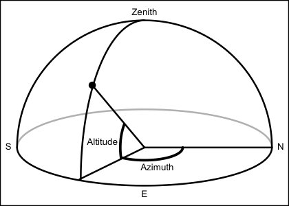
Alternate formulations

Formulae provide by Meeus (1982) are used for all calculations here. Meeus (1991) provides formulae that are similar, but that differ in the 5th or 6th digits. For example, the formula for ephemeris time in Meeus (1991) differs from that in Meeus (1992) at the 5th digit, and almost all of the approximately 200 coefficients in the relevant formulae also differ in the 5th and 6th digits. Discussion of the changing formulations is best left to members of the astronomical community. For the present purpose, it may be sufficient to note that moonAngle, based on Meeus (1982), reproduces the values provided in example 45.a of Meeus (1991) to 4 significant digits, e.g. with all angles matching to under 2 minutes of arc.

Author(s)

Dan Kelley, based on formulae in Meeus (1982).

References

Meeus, Jean. Astronomical Formulas for Calculators. Second Edition. Richmond, Virginia, USA: Willmann-Bell, 1982.
Meeus, Jean. Astronomical Algorithms. Second Edition. Richmond, Virginia, USA: Willmann-Bell, 1991.

Examples


library(oce)
par(mfrow = c(3, 2))
y <- 2012
m <- 4
days <- 1:3
# Halifax sunrise/sunset (see e.g. https://www.timeanddate.com/worldclock)
rises <- ISOdatetime(y, m, days, c(13, 15, 16), c(55, 04, 16), 0, tz = "UTC") + 3 * 3600 # ADT
sets <- ISOdatetime(y, m, days, c(3, 4, 4), c(42, 15, 45), 0, tz = "UTC") + 3 * 3600
azrises <- c(69, 75, 82)
azsets <- c(293, 288, 281)
latitude <- 44.65
longitude <- -63.6
for (i in 1:3) {
    t <- ISOdatetime(y, m, days[i], 0, 0, 0, tz = "UTC") + seq(0, 24 * 3600, 3600 / 4)
    ma <- moonAngle(t, longitude, latitude)
    oce.plot.ts(t, ma$altitude, type = "l", mar = c(2, 3, 1, 1), cex = 1 / 2, ylab = "Altitude")
    abline(h = 0)
    points(rises[i], 0, col = "red", pch = 3, lwd = 2, cex = 1.5)
    points(sets[i], 0, col = "blue", pch = 3, lwd = 2, cex = 1.5)
    oce.plot.ts(t, ma$azimuth, type = "l", mar = c(2, 3, 1, 1), cex = 1 / 2, ylab = "Azimuth")
    points(rises[i], -180 + azrises[i], col = "red", pch = 3, lwd = 2, cex = 1.5)
    points(sets[i], -180 + azsets[i], col = "blue", pch = 3, lwd = 2, cex = 1.5)
}

Convert a Numeric Time to Hour, Minute, and Second

Description

Convert a Numeric Time to Hour, Minute, and Second

Usage

numberAsHMS(t, default = 0)

Arguments

t

a vector of factors or character strings, in the format 1200 for 12:00, 0900 for 09:00, etc.

default

value to be used for the returned hour, minute and second if there is something wrong with the input value (e.g. its length exceeds 4 characters, or it contains non-numeric characters)

Value

A list containing hour, minute, and second, the last of which is always zero.

Author(s)

Dan Kelley

Examples

t <- c("0900", "1234")
numberAsHMS(t)

Convert a Numeric Time to a POSIXct Time

Description

This converts numerical values into POSIXct times. There are many schemes for doing this, with the type parameter being used to select between them. See “Details” for a listing, broken down by scheme.

Usage

numberAsPOSIXct(t, type = "unix", tz = "UTC", leap = TRUE)

Arguments

t

an integer corresponding to a time, in a way that depends on type.

type

character value indicating the time type. The permitted values are "argo", "epic", "excel", "gps", "matlab", "ncep1", "ncep2", "sas", "spss", "unix", and "yearday", the first of these being the default.

tz

a string indicating the time zone, by default "UTC".

leap

a logical value, TRUE by default, that applies only if type is "gps". If leap is TRUE, then the built-in dataset named .leap.seconds is consulted to find of the number of leap seconds between 1980 (when the GPS program started) and the time computed from the other parameters, and the return value is decreased accordingly (see Example 3).

Details

The possible choices for type are as listed below.

"unix" handles Unix times, measured in seconds since the start of the year 1970.
"matlab" handles Matlab times, measured in days since what MathWorks (reference 1) calls “January 0, 0000” (i.e. ISOdatetime(0, 1, 1, 0, 0, 0) in R notation).
"gps" handles the Global Positioning System convention. The scheme is complicated, owing to hardware limitations of GPS satellites. As illustrated in Example 3, t may be a matrix with either 2 or 3 columns. In the 2-column format, the first column holds the number of weeks after 1999-08-22, modulo 1024 (approximately 19.6 years), and the second column (here and also in the 3-column format) holds the number of seconds in the referenced week, with leap seconds being handled with the leap parameter. The modulo calculation is required because GPS satellites dedicate only 10 bits to the week number. The resultant ambiguity (e.g. a rollover in 2019-04-07) is addressed in the 3-column format, in which the last column holds the number of 1024-week rollover events since 1980-01-06. Users should set this column to 0 for times prior to 1999-08-22, to 1 for later times prior to 2019-04-07, to 2 for later times prior to 2038-11-21, etc. However, there will be an exception to this rule, when satellites start dedicating 12 bits to the week value. For such data, the third column will need to be 0 for all times prior to 2137-01-06.
"argo" handles Argo times, measured in days since the start of the year 1900.
"excel" handles Excel times, measured in days since the start of the year 1900. (Note that excel incorrectly regards 1900 as a leap year, so 1 day is subtracted from t unless the time is less than or equal to 1900 Feb 28. Note that NA is returned for the day 60, which is what excel codes for "Feb 29, 1900", the non-existing day that excel accepts.
"ncep1" handles NCEP times, measured in hours since the start of the year 1800.
"ncep2" handles NCEP times, measured in days since the start of the year 1. (Note that, for reasons that are unknown at this time, a simple R expression of this definition is out by two days compared with the UDUNITS library, which is used by NCEP. Therefore, a two-day offset is applied. See references 2 and 3.)
"sas" handles SAS times, indicated by type="sas", have origin at the start of 1960.
"spss" handles SPSS times, in seconds after 1582-10-14.
"yearday" handles a convention in which t is a two-column matrix, with the first column being the year, and the second the yearday (starting at 1 for the first second of January 1, to match the convention used by Sea-Bird CTD software).
"epic" handles a convention used in the EPIC software library, from the Pacific Marine Environmental Laboratory, in which t is a two-column matrix, with the first column being the julian Day (as defined in julianDay(), for example), and with the second column being the millisecond within that day. See reference 4.
"vms" handles a convention used in the VMS operating system and for Modified Julian Day, in which t is the number of seconds past 1859-11-17T00:00:00 UTC. See reference 5.

Value

A POSIXct() time vector.

Author(s)

Dan Kelley

References

Matlab times: ⁠https://www.mathworks.com/help/matlab/ref/datenum.html⁠
NCEP times: ⁠https://psl.noaa.gov/data/gridded/faq.html⁠
Problem with NCEP times: ⁠https://github.com/dankelley/oce/issues/738⁠
EPIC times: software and manuals at ⁠https://www.pmel.noaa.gov/epic/download/index.html#epslib⁠; see also Denbo, Donald W., and Nancy N. Soreide. “EPIC.” Oceanography 9 (1996). doi:10.5670/oceanog.1996.10
VMS times: https://en.wikipedia.org/wiki/Epoch_(computing)
GPS times: https://www.labsat.co.uk/index.php/en/gps-time-calculator

Examples

# Example 1. default (unix)
numberAsPOSIXct(0)

# Example 2. Matlab
numberAsPOSIXct(1, type = "matlab")

# Example 3. GPS with default week rollover or with no rollover (Canada Day, year 2010)
numberAsPOSIXct(cbind(566, 345615), type = "gps")
numberAsPOSIXct(cbind(566, 345615, 1), type = "gps")
numberAsPOSIXct(cbind(1024 + 566, 345615, 0), type = "gps")
# Show how to deal with leap seconds (15 of them, in this case)
sum(as.POSIXct("1980-01-01") < .leap.seconds & .leap.seconds <= as.POSIXct("2010-07-01"))
-15 + numberAsPOSIXct(cbind(1024 + 566, 345615, 0), type = "gps", leap = FALSE)

# Example 4. yearday
numberAsPOSIXct(cbind(2013, 1), type = "yearday") # start of 2013

# Example 5. Epic time, one hour into Canada Day of year 2018. In computing the
# Julian day, note that this starts at noon.
jd <- julianDay(as.POSIXct("2018-07-01 12:00:00", tz = "UTC"))
numberAsPOSIXct(cbind(jd, 1e3 * 1 * 3600), type = "epic", tz = "UTC")

# Example 6. Julian day, note that this starts at noon.
jd <- julianDay(as.POSIXct("2018-07-01 12:00:00", tz = "UTC"))
numberAsPOSIXct(cbind(jd, 1e3 * 1 * 3600), type = "epic", tz = "UTC")

Base Class for oce Objects

Description

This is mainly used within oce to create sub-classes, although users can use new("oce") to create a blank oce object, if desired.

Slots

metadata: A list containing information about the data. The contents vary across sub-classes, e.g. an adp object has information about beam patterns, which obviously would not make sense for a ctd object In addition, all classes have items named units and flags, used to store information on the units of the data, and the data quality.
data: A list containing the data.
processingLog: A list containing time-stamped processing steps, typically stored in the object by oce functions.

Examples

str(new("oce"))

Deprecated and Defunct Elements of the oce Package

Description

Certain functions and function arguments are still provided for compatibility with older versions of oce, but will be removed soon. The oce scheme for removing functions is similar to that used by Bioconductor: items are marked as "deprecated" in one release, marked as "defunct" in the next, and removed in the next after that. This goal is to provide a gentle migration path for users who keep their packages reasonably up-to-date.

Details

The following are marked "deprecated" in the present CRAN release of oce. Please use the replacement functions as listed below. The upcoming CRAN release of oce will mark these as "defunct", which is the last step before outright removal.

Deprecated	Replacement	Deprecated	Defunct	Removed

The following are marked "defunct", so calling them in the the present version produces an error message that hints at a replacement function. Once a function is marked "defunct" on one CRAN release, it will be slated for outright deletion in some subsequent release.

Defunct	Replacement	Version

The following functions were removed after having been marked as "deprecated" in at least one CRAN release, and possibly as "defunct" in at least one CRAN release. (The version number in the table is the first version to lack the named function.)

Function	Replacement	Version
`addColumn()`	`oceSetData()`	1.1-2
`ctdAddColumn()`	`oceSetData()`	1.1-2
`ctdUpdateHeader()`	`oceSetMetadata()`	1.1-2
`findInOrdered()`	`findInterval()`	1.1-2
`makeSection()`	`as.section()`	0.9.24
`mapMeridians()`	`mapGrid()`	1.1-2
`mapZones()`	`mapGrid()`	1.1-2
`oce.as.POSIXlt()`	`lubridate::parse_date_time()`	1.1-2
`renameData()`	`oceRenameData()`	1.7-9
`trimString()`	`trimws()`	1.8-2

Several “oce” function arguments are considered "defunct", which means they will be removed in the next CRAN release. They are as follows.

The fill argument of mapPlot() was confusing to users, so it was designated as deprecated in June 2016. (The confusion stemmed from subtle differences between plot() and polygon(), and the problem is that mapPlot() can use either of these functions, according to whether coastlines are to be filled.) The functionality is preserved, in the col argument.

Version of as.raw() That Clips Data

Description

A version of as.raw() that clips data to prevent warnings

Usage

oce.as.raw(x)

Arguments

x

values to be converted to raw

Details

Negative values are clipped to 0, while values above 255 are clipped to 255; the result is passed to as.raw() and returned.

Value

Raw values corresponding to x.

Author(s)

Dan Kelley

Examples

x <- c(-0.1, 0, 1, 255, 255.1)
data.frame(x, oce.as.raw(x))

Oce Version of axis.POSIXct

Description

A specialized variant of axis.POSIXct() that produces results with less ambiguity in axis labels.

Usage

oce.axis.POSIXct(
  side,
  x,
  at,
  tformat,
  labels = TRUE,
  drawTimeRange,
  abbreviateTimeRange = FALSE,
  drawFrequency = FALSE,
  cex.axis = par("cex.axis"),
  cex.lab = par("cex.lab"),
  cex.main = par("cex.main"),
  mar = par("mar"),
  mgp = par("mgp"),
  main = "",
  debug = getOption("oceDebug"),
  ...
)

Arguments

side

as for axis.POSIXct().

x

as for axis.POSIXct().

at

as for axis.POSIXct().

tformat

as format for axis.POSIXct() for now, but may eventually have new features for multiline labels, e.g. day on one line and month on another.

labels

as for axis.POSIXct().

drawTimeRange

Optional indication of whether/how to draw the time range in the margin on the side of the the plot opposite the time axis. If this is not supplied, it defaults to the value returned by getOption("oceDrawTimeRange"), and if that option is not set, it defaults to TRUE. No time range is drawn if drawTimeRange is FALSE. If it is TRUE, the range will be shown. This range refers to range of the x axis (not the data). The format of the elements of that range is set by getOption("oceTimeFormat") (or with the default value of an empty string, if this option has not been set). The timezone will be indicated if the time range is under a week. For preliminary work, it makes sense to use drawTimeRange=TRUE, but for published work it can be better to drop this label and indicate something about the time in the figure caption.

abbreviateTimeRange

boolean, TRUE to abbreviate the second number in the time range, e.g. dropping the year if it is the same in the first number.

drawFrequency

boolean, TRUE to show the frequency of sampling in the data

cex.axis, cex.lab, cex.main

character expansion factors for axis numbers, axis names and plot titles; see par().

mar

value for par(mar) for axis

mgp

value for par(mgp) for axis

main

title of plot

debug

a flag that turns on debugging. Set to 1 to get a moderate amount of debugging information, or to 2 to get more.

...

as for axis.POSIXct().

Details

The tick marks are set automatically based on examination of the time range on the axis. The scheme was devised by constructing test cases with a typical plot size and font size, and over a wide range of time scales. In some categories, both small tick marks are interspersed between large ones.

The user may set the format of axis numbers with the tformat argument. If this is not supplied, the format is set based on the time span of the axis:

If this time span is less than a minute, the time axis labels are in seconds (fractional seconds, if the interval is less than 2 seconds), with leading zeros on small integers. (Fractional seconds are enabled with a trick: the usual R format "\%S" is supplemented with a new format e.g. "\%.2S", meaning to use two digits after the decimal.)
If the time span exceeds a minute but is less than 1.5 days, the label format is "\%H:\%M:\%S".
If the time span exceeds 1.5 days but is less than 1 year, the format is "\%b \%d" (e.g. Jul 15) and, again, the tick marks are set up for several subcategories.
If the time span exceeds a year, the format is "\%Y", i.e. the year is displayed with 4 digits.

It should be noted that this scheme differs from the R approach in several ways. First, R writes day names for some time ranges, in a convention that is seldom seen in the literature. Second, R will write nn:mm for both HH:MM and MM:SS, an ambiguity that might confuse readers. Third, the use of both large and small tick marks is not something that R does.

Bear in mind that tformat may be set to alter the number format, but that the tick mark scheme cannot (presently) be controlled.

Value

A vector of times corresponding to axis ticks is returned silently.

Author(s)

Dan Kelley

Oce Variant of contour

Description

This provides something analogous to contour(), but with the ability to flip x and y. Setting revy=TRUE can be helpful if the y data represent pressure or depth below the surface.

Usage

oce.contour(
  x,
  y,
  z,
  revx = FALSE,
  revy = FALSE,
  add = FALSE,
  tformat,
  drawTimeRange = getOption("oceDrawTimeRange"),
  debug = getOption("oceDebug"),
  ...
)

Arguments

x

values for x grid.

y

values for y grid.

z

matrix for values to be contoured. The first dimension of z must equal the number of items in x, etc.

revx

set to TRUE to reverse the order in which the labels on the x axis are drawn

revy

set to TRUE to reverse the order in which the labels on the y axis are drawn

add

logical value indicating whether the contours should be added to a pre-existing plot.

tformat

time format; if not supplied, a reasonable choice will be made by oce.axis.POSIXct(), which draws time axes.

drawTimeRange

logical, only used if the x axis is a time. If TRUE, then an indication of the time range of the data (not the axis) is indicated at the top-left margin of the graph. This is useful because the labels on time axes only indicate hours if the range is less than a day, etc.

debug

a flag that turns on debugging; set to 1 to information about the processing.

...

optional arguments passed to plotting functions.

Author(s)

Dan Kelley

Examples

library(oce)
data(topoWorld)
# coastline now, and in last glacial maximum
lon <- topoWorld[["longitude"]]
lat <- topoWorld[["latitude"]]
z <- topoWorld[["z"]]
oce.contour(lon, lat, z, levels = 0, drawlabels = FALSE)
oce.contour(lon, lat, z, levels = -130, drawlabels = FALSE, col = "blue", add = TRUE)

Add a Grid to an Existing Oce Plot

Description

Add a Grid to an Existing Oce Plot

Usage

oce.grid(xat, yat, col = "lightgray", lty = "dotted", lwd = par("lwd"))

Arguments

xat

either a list of x values at which to draw the grid, or the return value from an oce plotting function

yat

a list of y values at which to plot the grid (ignored if gx was a return value from an oce plotting function)

col

color of grid lines (see par())

lty

type for grid lines (see par())

lwd

width for grid lines (see par())

Details

For plots not created by oce functions, or for missing xat and yat, this is the same as a call to grid() with missing nx and ny. However, if xat is the return value from certain oce functions, a more sophisticated grid is constructed. The problem with grid() is that it cannot handle axes with non-uniform grids, e.g. those with time axes that span months of differing lengths.

As of early February 2015, oce.grid handles xat produced as the return value from the following functions: imagep() and oce.plot.ts(), plot,adp-method(), plot,echosounder-method(), and plotTS(). It makes no sense to try to use oce.grid for multipanel oce plots, e.g. the default plot from plot,adp-method().

Examples

library(oce)
i <- imagep(volcano)
oce.grid(i, lwd = 2)

data(sealevel)
i <- oce.plot.ts(sealevel[["time"]], sealevel[["elevation"]])
oce.grid(i, col = "red")

data(ctd)
i <- plotTS(ctd)
oce.grid(i, col = "red")

data(adp)
i <- plot(adp, which = 1)
oce.grid(i, col = "gray", lty = 1)

data(echosounder)
i <- plot(echosounder)
oce.grid(i, col = "pink", lty = 1)

Oce Variant of plot.ts

Description

Plot a time-series, obeying the timezone and possibly drawing the range in the top-left margin.

Usage

oce.plot.ts(
  x,
  y,
  type = "l",
  xlim,
  ylim,
  log = "",
  logStyle = "r",
  flipy = FALSE,
  xlab,
  ylab,
  drawTimeRange,
  simplify = 2560,
  fill = FALSE,
  col = par("col"),
  pch = par("pch"),
  cex = par("cex"),
  cex.axis = par("cex.axis"),
  cex.lab = par("cex.lab"),
  cex.main = par("cex.main"),
  xaxs = par("xaxs"),
  yaxs = par("yaxs"),
  mgp = getOption("oceMgp"),
  mar = c(mgp[1] + if (nchar(xlab) > 0) 1.5 else 1, mgp[1] + 1.5, mgp[2] + 1, mgp[2] +
    3/4),
  main = "",
  despike = FALSE,
  axes = TRUE,
  tformat,
  marginsAsImage = FALSE,
  grid = FALSE,
  grid.col = "lightgray",
  grid.lty = "dotted",
  grid.lwd = par("lwd"),
  debug = getOption("oceDebug"),
  ...
)

Arguments

x

the times of observations. If this is not a POSIXt object, then an attempt is made to convert it to one using as.POSIXct().

y

the observations.

type

plot type, "l" for lines, "p" for points.

xlim

optional limit for x axis. This has an additional effect, beyond that for conventional R functions: it effectively windows the data, so that autoscaling will yield limits for y that make sense within the window.

ylim

optional limit for y axis.

log

a character value that must be either empty (the default) for linear y axis, or "y" for logarithmic y axis. (Unlike plot.default() etc., oce.plot.ts does not permit logarithmic time, or x axis.)

logStyle

a character value that indicates how to draw the y axis, if log="y". If it is "r" (the default) then the conventional R style is used, in which a logarithmic transform connects y values to position on the "page" of the plot device, so that tics will be nonlinearly spaced, but not organized by integral powers of 10. However, if it is "decade", then the style will be that used in the scientific literature, in which large tick marks are used for integral powers of 10, with smaller tick marks at integral multiples of those powers, and with labels that use exponential format for values above 100 or below 0.01. The value of logStyle is passed to oceAxis(), which draws the axis.

flipy

Logical, with TRUE indicating that the graph should have the y axis reversed, i.e. with smaller values at the bottom of the page.

xlab

name for x axis; defaults to "".

ylab

name for y axis; defaults to the plotted item.

drawTimeRange

an optional indication of whether/how to draw a time range, in the top-left margin of the plot; see oce.axis.POSIXct() for details.

simplify

an integer value that indicates whether to speed up type="l" plots by replacing the data with minimum and maximum values within a subsampled time mesh. This can speed up plots of large datasets (e.g. by factor 20 for 10^7 points), sometimes with minor changes in appearance. This procedure is skipped if simplify is NA or if the number of visible data points is less than 5 times simplify. Otherwise, oce.plot.ts creates simplify intervals ranging across the visible time range. Intervals with under 2 finite y data are ignored. In the rest, y values are replaced with their range, and x values are replaced with the repeated midpoint time. Thus, each retained sub-interval has exactly 2 data points. A warning is printed if this replacement is done. The default value of simplify means that cases with under 2560 visible points are plotted conventionally.

fill

boolean, set TRUE to fill the curve to zero (which it does incorrectly if there are missing values in y).

col

The colours for points (if type=="p") or lines (if type=="l"). For the type="p" case, if there are fewer col values than there are x values, then the col values are recycled in the standard fashion. For the type="l" case, the line is plotted in the first colour specified.

pch

character code, used if type=="p". If there are fewer pch values than there are x values, then the pch values are recycled in the standard fashion. See points() for the possible values for pch.

cex

numeric character expansion factor for points on plots, ignored unless type is "p". This may be a single number, applied to all points, or a vector of numbers to be applied to the points in sequence. If there are fewer pch values than there are x values, then the pch values are recycled in the standard fashion. See par() for more on cex.

cex.axis, cex.lab, cex.main

numeric character expansion factors for axis numbers, axis names and plot titles; see par().

xaxs

control x axis ending; see par("xaxs").

yaxs

control y axis ending; see par("yaxs").

mgp

3-element numerical vector to use for par(mgp), and also for par(mar), computed from this. The default is tighter than the R default, in order to use more space for the data and less for the axes.

mar

value to be used with par("mar") to set margins. The default value uses significantly tighter margins than is the norm in R, which gives more space for the data. However, in doing this, the existing par("mar") value is ignored, which contradicts values that may have been set by a previous call to drawPalette(). To get plot with a palette, first call drawPalette(), then call oce.plot.ts with mar=par("mar").

main

title of plot.

despike

boolean flag that can turn on despiking with despike().

axes

boolean, set to TRUE to get axes plotted

tformat

optional format for labels on the time axis

marginsAsImage

boolean indicating whether to set the right-hand margin to the width normally taken by an image drawn with imagep().

grid

if TRUE, a grid will be drawn for each panel. (This argument is needed, because calling grid() after doing a sequence of plots will not result in useful results for the individual panels.

grid.col

color of grid

grid.lty

line type of grid

grid.lwd

line width of grid

debug

a flag that turns on debugging. Set to 1 to get a moderate amount of debugging information, or to 2 to get more.

...

graphical parameters passed down to plot().

Details

Depending on the version of R, the standard plot() and plot.ts() routines will not obey the time zone of the data. This routine gets around that problem. It can also plot the time range in the top-left margin, if desired; this string includes the timezone, to remove any possible confusion. The time axis is drawn with oce.axis.POSIXct().

Value

A list is silently returned, containing xat and yat, values that can be used by oce.grid() to add a grid to the plot.

Author(s)

Dan Kelley and Clark Richards

Examples

library(oce)
t0 <- as.POSIXct("2008-01-01", tz = "UTC")
t <- seq(t0, length.out = 48, by = "30 min")
y <- sin(as.numeric(t - t0) * 2 * pi / (12 * 3600))
oce.plot.ts(t, y, type = "l", xaxs = "i")
# Show how col, pch and cex get recycled
oce.plot.ts(t, y,
    type = "p", xaxs = "i",
    col = 1:3, pch = c(rep(1, 6), rep(20, 6)), cex = sqrt(1:6)
)
# Trimming x; note the narrowing of the y view
oce.plot.ts(t, y, type = "p", xlim = c(t[6], t[12]))
# Flip the y axis
oce.plot.ts(t, y, flipy = TRUE)

Write the Data Portion of Object to a File

Description

The output has a line containing the names of the columns in x$data, each enclosed in double quotes. After that line are lines for the data themselves. The default is to separate data items by a single space character, but this can be altered by using a sep argument in the ... list; see utils::write.table().

Usage

oce.write.table(x, file = "", ...)

Arguments

x

an oce object.

file

file name, as passed to utils::write.table(). Use "" to get a listing in the terminal window.

...

optional arguments passed to utils::write.table().

Details

This function is little more than a thin wrapper around utils::write.table(), the only difference being that row names are omitted here, making for a file format that is more conventional in Oceanography.

Value

The value returned by utils::write.table().

Author(s)

Dan Kelley

Interpolate 1D Data with UNESCO or Reiniger-Ross Algorithm

Description

Interpolate one-dimensional data using schemes that permit curvature but tends minimize extrema that are not well-indicated by the data.

Usage

oceApprox(x, y, xout, method = c("rr", "unesco"))

Arguments

x

the independent variable (z or p, usually).

y

the dependent variable.

xout

the values of the independent variable at which interpolation is to be done.

method

method to use. See “Details”.

Details

Setting method="rr" yields the weighted-parabola algorithm of Reiniger and Ross (1968). For procedure is as follows. First, the interpolant for any xout value that is outside the range of x is set to NA. Next, linear interpolation is used for any xout value that has only one smaller neighboring x value, or one larger neighboring value. For all other values of xout, the 4 neighboring points x are sought, two smaller and two larger. Then two parabolas are determined, one from the two smaller points plus the nearest larger point, and the other from the nearest smaller point and the two larger points. A weighted sum of these two parabolas provides the interpolated value. Note that, in the notation of Reiniger and Ross (1968), this algorithm uses m=2 and n=1. (A future version of this routine might provide the ability to modify these values.)

Setting method="unesco" yields the method that is used by the U.S. National Oceanographic Data Center. It is described in pages 48-50 of reference 2; reference 3 presumably contains the same information but it is not as easily accessible. The method works as follows.

If there are data above 5m depth, then the surface value is taken to equal to the shallowest recorded value.
Distance bounds are put on the four neighboring points, and the Reiniger-Ross method is used for interpolated points with sufficiently four close neighbors. The bounds are described in table 15 of reference 2 only for so-called standard depths; in the present instance they are transformed to the following rules. Inner neighbors must be within 5m for data above 10m, 50m above 250m 100m above 900m, 200m above 2000m, or within 1000m otherwise. Outer neighbors must be within 200m above 500m, 400m above 1300m, or 1000m otherwise. If two or more points meet these criteria, Lagrangian interpolation is used. If not, NA is used as the interpolant.

After these rules are applied, the interpolated value is compared with the values immediately above and below it, and if it is outside the range, simple linear interpolation is used.

Value

A vector of interpolated values, corresponding to the xout values and equal in number.

Author(s)

Dan Kelley

References

R.F. Reiniger and C.K. Ross, 1968. A method of interpolation with application to oceanographic data. Deep Sea Research, 15, 185-193.
Daphne R. Johnson, Tim P. Boyer, Hernan E. Garcia, Ricardo A. Locarnini, Olga K. Baranova, and Melissa M. Zweng, 2011. World Ocean Database 2009 Documentation. NODC Internal report 20. Ocean Climate Laboratory, National Oceanographic Data Center. Silver Spring, Maryland.
UNESCO, 1991. Processing of oceanographic station data, 138 pp., Imprimerie des Presses Universitaires de France, United Nations Educational, Scientific and Cultural Organization, France.

Examples

library(oce)
if (require(ocedata)) {
    data(RRprofile)
    zz <- seq(0, 2000, 2)
    plot(RRprofile$temperature, RRprofile$depth, ylim = c(500, 0), xlim = c(2, 11))
    # Contrast two methods
    a1 <- oce.approx(RRprofile$depth, RRprofile$temperature, zz, "rr")
    a2 <- oce.approx(RRprofile$depth, RRprofile$temperature, zz, "unesco")
    lines(a1, zz)
    lines(a2, zz, col = "red")
    legend("bottomright", lwd = 1, col = 1:2, legend = c("rr", "unesco"), cex = 3 / 4)
}

Draw an Axis, Possibly with Decade-style Logarithmic Scaling

Description

Draw an Axis, Possibly with Decade-style Logarithmic Scaling

Usage

oceAxis(side, labels = TRUE, logStyle = "r", ...)

Arguments

side

an integer specifying which axis to draw, with 1 for bottom axis, 2 for left axis, 3 for top axis, and 4 for right axis (as with axis()).

labels

either a vector of character values used for labels or a logical value indicating whether to draw such labels. The first form only works if the coordinate is not logarithmic, and if logStyle is "r".

logStyle

...

other graphical parameters, passed to axis().

Value

Numerical values at which tick marks were drawn (or would have been drawn, if labels specified to draw them).

Author(s)

Dan Kelley

Examples

library(oce)
Ra <- 10^seq(4, 10, 0.1)
Nu <- 0.085 * Ra^(1 / 3)
plot(Ra, Nu, log = "xy", axes = FALSE)
box()
oceAxis(1, logStyle = "decade")
oceAxis(2, logStyle = "decade")

Coordinate Reference System Strings for Some Oceans

Description

Create a coordinate reference string (CRS), suitable for use as a projection argument to mapPlot() or plot,coastline-method().

Usage

oceCRS(region)

Arguments

region

character string indicating the region. This must be in the following list (or a string that matches to just one entry, with pmatch()): "North Atlantic", "South Atlantic", "Atlantic", "North Pacific", "South Pacific", "Pacific", "Arctic", and "Antarctic".

Value

string contain a CRS, which can be used as projection in mapPlot().

Caution

This is a preliminary version of this function, with the results being very likely to change through the autumn of 2016, guided by real-world usage.

Author(s)

Dan Kelley

Examples


library(oce)
data(coastlineWorld)
par(mar = c(2, 2, 1, 1))
plot(coastlineWorld, projection = oceCRS("Atlantic"), span = 12000)
plot(coastlineWorld, projection = oceCRS("North Atlantic"), span = 8000)
plot(coastlineWorld, projection = oceCRS("South Atlantic"), span = 8000)
plot(coastlineWorld, projection = oceCRS("Arctic"), span = 4000)
plot(coastlineWorld, projection = oceCRS("Antarctic"), span = 10000)
# Avoid ugly horizontal lines, an artifact of longitude shifting.
# Note: we cannot fill the land once we shift, either.
pacific <- coastlineCut(coastlineWorld, -180)
plot(pacific, proj = oceCRS("Pacific"), span = 15000, col = NULL)
plot(pacific, proj = oceCRS("North Pacific"), span = 12000, col = NULL)
plot(pacific, proj = oceCRS("South Pacific"), span = 12000, col = NULL)

Create Colors in a Red-Yellow-Blue Color Scheme

Description

The results are similar to those of oceColorsJet(), but with white hues in the centre, rather than green ones. The scheme may be useful in displaying signed quantities, and thus is somewhat analogous to oceColorsTwo(), except that some viewers may be able to distinguish more colors with oceColors9B.

Usage

oceColors9B(n)

Arguments

n

number of colors

References

The following references provide information on choosing colour schemes, that are suitable for viewers who have colour deficiencies.

Examples

library(oce)
imagep(volcano,
    col = oceColors9B(128),
    zlab = "oceColors9B"
)

Create Colors Suitable for CDOM Fields

Description

Create a set of colors for displaying CDOM values, based on the scheme devised by Thyng et al. (2016) and presented in a python package by Thyng (2019). The color specifications were transliterated from python to R on 2015-09-29, but have not been adjusted since, even though the python source has changed. This is to prevent breaking old oce code. To get the latest versions of these colours or other colours, use the cmocean R package (Thyng, Richards, and Krylov, 2019) directly, as is illustrated (with the "matter" scheme) in Example 2. Note that the cmocean core functions provide a way to select between various versions of the colour schemes. It is also worth considering the palettes provided by the viridis package, as illustrated (with the "inferno" scheme) in Example 3.

Usage

oceColorsCDOM(n)

Arguments

n

number of colors to create.

Value

A vector of color specifications.

Author(s)

Krysten M. Thyng (Python version), Dan Kelley (R transliteration)

References

Thyng, Kristen, Chad Greene, Robert Hetland, Heather Zimmerle, and Steven DiMarco. “True Colors of Oceanography: Guidelines for Effective and Accurate Colormap Selection.” Oceanography 29, no. 3 (September 1, 2016): 9–13. doi:10.5670/oceanog.2016.66
Thyng, Kristen. Kthyng/Cmocean. Python, 2019. ⁠https://github.com/kthyng/cmocean⁠.
Thyng, Kristen, Clark Richards, and Ivan Krylov. Cmocean: Beautiful Colour Maps for Oceanography (version 0.2), 2019. ⁠https://CRAN.R-project.org/package=cmocean⁠.

The following references provide information on choosing colour schemes, that are suitable for viewers who have colour deficiencies.

Examples

library(oce)

# Example 1
imagep(volcano, col=oceColorsCDOM(128),
    zlab="oceColorsCDOM")
## Not run: 
# Example 2 (requires the cmocean package)
imagep(volcano, col=cmocean::cmocean("matter"),
    zlab="cmocean::cmocean(\"matter\")")
## End(Not run)

## Not run: 
# Example 3 (requires the viridis package)
imagep(volcano, col=viridis::inferno,
    zlab="viridis::inferno")
## End(Not run)

Create Colors Suitable for chlorophyll Fields

Description

Create a set of colors for displaying chlorophyll values, based on the scheme devised by Thyng et al. (2016) and presented in a python package by Thyng (2019). The color specifications were transliterated from python to R on 2015-09-29, but have not been adjusted since, even though the python source has changed. This is to prevent breaking old oce code. To get the latest versions of these colours or other colours, use the cmocean R package (Thyng, Richards, and Krylov, 2019) directly, as is illustrated (with the "matter" scheme) in Example 2. Note that the cmocean core functions provide a way to select between various versions of the colour schemes. It is also worth considering the palettes provided by the viridis package, as illustrated (with the "inferno" scheme) in Example 3.

Usage

oceColorsChlorophyll(n)

Arguments

n

number of colors to create.

Value

A vector of color specifications.

Author(s)

Krysten M. Thyng (Python version), Dan Kelley (R transliteration)

References

Thyng, Kristen, Chad Greene, Robert Hetland, Heather Zimmerle, and Steven DiMarco. “True Colors of Oceanography: Guidelines for Effective and Accurate Colormap Selection.” Oceanography 29, no. 3 (September 1, 2016): 9–13. doi:10.5670/oceanog.2016.66
Thyng, Kristen. Kthyng/Cmocean. Python, 2019. ⁠https://github.com/kthyng/cmocean⁠.
Thyng, Kristen, Clark Richards, and Ivan Krylov. Cmocean: Beautiful Colour Maps for Oceanography (version 0.2), 2019. ⁠https://CRAN.R-project.org/package=cmocean⁠.

The following references provide information on choosing colour schemes, that are suitable for viewers who have colour deficiencies.

Examples

library(oce)

# Example 1
imagep(volcano, col=oceColorsChlorophyll(128),
    zlab="oceColorsChlorophyll")
## Not run: 
# Example 2 (requires the cmocean package)
imagep(volcano, col=cmocean::cmocean("matter"),
    zlab="cmocean::cmocean(\"matter\")")
## End(Not run)

## Not run: 
# Example 3 (requires the viridis package)
imagep(volcano, col=viridis::inferno,
    zlab="viridis::inferno")
## End(Not run)

Create Color Functions

Description

This function generates other functions that are used to specify colors. It is used within oce to create oceColorsTemperature() and its many cousins. Users may also find it helpful, for creating custom color schemes (see “Examples”).

Usage

oceColorsClosure(spec)

Arguments

spec

Specification of the color scheme. This may be a character string, in which case it must be the name of an item stored in data(ocecolors), or either a 3-column data frame or matrix, in which case the columns specify red, green and blue values (in range from 0 to 1).

Sample of Usage

# Update oxygen color scheme to latest matplotlib value.
library(oce)
oxy <- "https://raw.githubusercontent.com/matplotlib/cmocean/master/cmocean/rgb/oxy-rgb.txt"
oxyrgb <- read.table(oxy, header=FALSE)
oceColorsOxygenUpdated <- oceColorsClosure(oxyrgb)
par(mfrow=c(1, 2))
m <- matrix(1:256)
imagep(m, col=oceColorsOxygen, zlab="oxygen")
imagep(m, col=oceColorsOxygenUpdated, zlab="oxygenUpdated")

Create Colors Suitable for density Fields

Description

Create a set of colors for displaying density values, based on the scheme devised by Thyng et al. (2016) and presented in a python package by Thyng (2019). The color specifications were transliterated from python to R on 2015-09-29, but have not been adjusted since, even though the python source has changed. This is to prevent breaking old oce code. To get the latest versions of these colours or other colours, use the cmocean R package (Thyng, Richards, and Krylov, 2019) directly, as is illustrated (with the "matter" scheme) in Example 2. Note that the cmocean core functions provide a way to select between various versions of the colour schemes. It is also worth considering the palettes provided by the viridis package, as illustrated (with the "inferno" scheme) in Example 3.

Usage

oceColorsDensity(n)

Arguments

n

number of colors to create.

Value

A vector of color specifications.

Author(s)

Krysten M. Thyng (Python version), Dan Kelley (R transliteration)

References

Thyng, Kristen, Chad Greene, Robert Hetland, Heather Zimmerle, and Steven DiMarco. “True Colors of Oceanography: Guidelines for Effective and Accurate Colormap Selection.” Oceanography 29, no. 3 (September 1, 2016): 9–13. doi:10.5670/oceanog.2016.66
Thyng, Kristen. Kthyng/Cmocean. Python, 2019. ⁠https://github.com/kthyng/cmocean⁠.
Thyng, Kristen, Clark Richards, and Ivan Krylov. Cmocean: Beautiful Colour Maps for Oceanography (version 0.2), 2019. ⁠https://CRAN.R-project.org/package=cmocean⁠.

The following references provide information on choosing colour schemes, that are suitable for viewers who have colour deficiencies.

Examples

library(oce)

# Example 1
imagep(volcano, col=oceColorsDensity(128),
    zlab="oceColorsDensity")
## Not run: 
# Example 2 (requires the cmocean package)
imagep(volcano, col=cmocean::cmocean("matter"),
    zlab="cmocean::cmocean(\"matter\")")
## End(Not run)

## Not run: 
# Example 3 (requires the viridis package)
imagep(volcano, col=viridis::inferno,
    zlab="viridis::inferno")
## End(Not run)

Create Colors Suitable for freesurface Fields

Description

Create a set of colors for displaying freesurface values, based on the scheme devised by Thyng et al. (2016) and presented in a python package by Thyng (2019). The color specifications were transliterated from python to R on 2015-09-29, but have not been adjusted since, even though the python source has changed. This is to prevent breaking old oce code. To get the latest versions of these colours or other colours, use the cmocean R package (Thyng, Richards, and Krylov, 2019) directly, as is illustrated (with the "matter" scheme) in Example 2. Note that the cmocean core functions provide a way to select between various versions of the colour schemes. It is also worth considering the palettes provided by the viridis package, as illustrated (with the "inferno" scheme) in Example 3.

Usage

oceColorsFreesurface(n)

Arguments

n

number of colors to create.

Value

A vector of color specifications.

Author(s)

Krysten M. Thyng (Python version), Dan Kelley (R transliteration)

References

Thyng, Kristen, Chad Greene, Robert Hetland, Heather Zimmerle, and Steven DiMarco. “True Colors of Oceanography: Guidelines for Effective and Accurate Colormap Selection.” Oceanography 29, no. 3 (September 1, 2016): 9–13. doi:10.5670/oceanog.2016.66
Thyng, Kristen. Kthyng/Cmocean. Python, 2019. ⁠https://github.com/kthyng/cmocean⁠.
Thyng, Kristen, Clark Richards, and Ivan Krylov. Cmocean: Beautiful Colour Maps for Oceanography (version 0.2), 2019. ⁠https://CRAN.R-project.org/package=cmocean⁠.

The following references provide information on choosing colour schemes, that are suitable for viewers who have colour deficiencies.

Examples

library(oce)

# Example 1
imagep(volcano, col=oceColorsFreesurface(128),
    zlab="oceColorsFreesurface")
## Not run: 
# Example 2 (requires the cmocean package)
imagep(volcano, col=cmocean::cmocean("matter"),
    zlab="cmocean::cmocean(\"matter\")")
## End(Not run)

## Not run: 
# Example 3 (requires the viridis package)
imagep(volcano, col=viridis::inferno,
    zlab="viridis::inferno")
## End(Not run)

Create Colors in a GEBCO-like Scheme

Description

The colours were determined by examination of paper charts printed during the GEBCO Fifth Edition era. The hues range from dark blue to light blue, then from light brown to dark brown. If used to show topography in scheme centred on z=0, this means that near-coastal regions are light in tone, with darker colours representing both mountains and the deep sea.

Usage

oceColorsGebco(
  n = 9,
  region = c("water", "land", "both"),
  type = c("fill", "line"),
  debug = getOption("oceDebug")
)

Arguments

n

Number of colors to return

region

String indicating application region, one of "water", "land", or "both".

type

String indicating the purpose, one of "fill" or "line".

debug

a flag that turns on debugging.

Examples

library(oce)
imagep(volcano, col = oceColorsGebco(128, region = "both"))

Create Colors Similar to the Matlab Jet Scheme

Description

Create Colors Similar to the Matlab Jet Scheme

Usage

oceColorsJet(n)

Arguments

n

number of colors

References

The following references provide information on choosing colour schemes, that are suitable for viewers who have colour deficiencies.

Examples

library(oce)
imagep(volcano, col = oceColorsJet, zlab = "oceColorsJet")

Create Colors Suitable for oxygen Fields

Description

Create a set of colors for displaying oxygen values, based on the scheme devised by Thyng et al. (2016) and presented in a python package by Thyng (2019). The color specifications were transliterated from python to R on 2015-09-29, but have not been adjusted since, even though the python source has changed. This is to prevent breaking old oce code. To get the latest versions of these colours or other colours, use the cmocean R package (Thyng, Richards, and Krylov, 2019) directly, as is illustrated (with the "matter" scheme) in Example 2. Note that the cmocean core functions provide a way to select between various versions of the colour schemes. It is also worth considering the palettes provided by the viridis package, as illustrated (with the "inferno" scheme) in Example 3.

Usage

oceColorsOxygen(n)

Arguments

n

number of colors to create.

Value

A vector of color specifications.

Author(s)

Krysten M. Thyng (Python version), Dan Kelley (R transliteration)

References

Thyng, Kristen, Chad Greene, Robert Hetland, Heather Zimmerle, and Steven DiMarco. “True Colors of Oceanography: Guidelines for Effective and Accurate Colormap Selection.” Oceanography 29, no. 3 (September 1, 2016): 9–13. doi:10.5670/oceanog.2016.66
Thyng, Kristen. Kthyng/Cmocean. Python, 2019. ⁠https://github.com/kthyng/cmocean⁠.
Thyng, Kristen, Clark Richards, and Ivan Krylov. Cmocean: Beautiful Colour Maps for Oceanography (version 0.2), 2019. ⁠https://CRAN.R-project.org/package=cmocean⁠.

The following references provide information on choosing colour schemes, that are suitable for viewers who have colour deficiencies.

Examples

library(oce)

# Example 1
imagep(volcano, col=oceColorsOxygen(128),
    zlab="oceColorsOxygen")
## Not run: 
# Example 2 (requires the cmocean package)
imagep(volcano, col=cmocean::cmocean("matter"),
    zlab="cmocean::cmocean(\"matter\")")
## End(Not run)

## Not run: 
# Example 3 (requires the viridis package)
imagep(volcano, col=viridis::inferno,
    zlab="viridis::inferno")
## End(Not run)

Create Colors Suitable for PAR Fields

Description

Create a set of colors for displaying PAR values, based on the scheme devised by Thyng et al. (2016) and presented in a python package by Thyng (2019). The color specifications were transliterated from python to R on 2015-09-29, but have not been adjusted since, even though the python source has changed. This is to prevent breaking old oce code. To get the latest versions of these colours or other colours, use the cmocean R package (Thyng, Richards, and Krylov, 2019) directly, as is illustrated (with the "matter" scheme) in Example 2. Note that the cmocean core functions provide a way to select between various versions of the colour schemes. It is also worth considering the palettes provided by the viridis package, as illustrated (with the "inferno" scheme) in Example 3.

Usage

oceColorsPAR(n)

Arguments

n

number of colors to create.

Value

A vector of color specifications.

Author(s)

Krysten M. Thyng (Python version), Dan Kelley (R transliteration)

References

Thyng, Kristen, Chad Greene, Robert Hetland, Heather Zimmerle, and Steven DiMarco. “True Colors of Oceanography: Guidelines for Effective and Accurate Colormap Selection.” Oceanography 29, no. 3 (September 1, 2016): 9–13. doi:10.5670/oceanog.2016.66
Thyng, Kristen. Kthyng/Cmocean. Python, 2019. ⁠https://github.com/kthyng/cmocean⁠.
Thyng, Kristen, Clark Richards, and Ivan Krylov. Cmocean: Beautiful Colour Maps for Oceanography (version 0.2), 2019. ⁠https://CRAN.R-project.org/package=cmocean⁠.

The following references provide information on choosing colour schemes, that are suitable for viewers who have colour deficiencies.

Examples

library(oce)

# Example 1
imagep(volcano, col=oceColorsPAR(128),
    zlab="oceColorsPAR")
## Not run: 
# Example 2 (requires the cmocean package)
imagep(volcano, col=cmocean::cmocean("matter"),
    zlab="cmocean::cmocean(\"matter\")")
## End(Not run)

## Not run: 
# Example 3 (requires the viridis package)
imagep(volcano, col=viridis::inferno,
    zlab="viridis::inferno")
## End(Not run)

Create a Vector of Colors

Description

The available schemes are:

which=1 for a red-white-blue scheme.
which=2 for a red-yellow-blue scheme.
which=9.01, which="9A" or which="jet" for oceColorsJet(n).
which=9.02 or which="9B" for oceColors9B(n).

Usage

oceColorsPalette(n, which = 1)

Arguments

n

number of colors to create

which

integer or character string indicating the palette to use; see “Details”.

References

The following references provide information on choosing colour schemes, that are suitable for viewers who have colour deficiencies.

Create Colors Suitable for phase Fields

Description

Create a set of colors for displaying phase values, based on the scheme devised by Thyng et al. (2016) and presented in a python package by Thyng (2019). The color specifications were transliterated from python to R on 2015-09-29, but have not been adjusted since, even though the python source has changed. This is to prevent breaking old oce code. To get the latest versions of these colours or other colours, use the cmocean R package (Thyng, Richards, and Krylov, 2019) directly, as is illustrated (with the "matter" scheme) in Example 2. Note that the cmocean core functions provide a way to select between various versions of the colour schemes. It is also worth considering the palettes provided by the viridis package, as illustrated (with the "inferno" scheme) in Example 3.

Usage

oceColorsPhase(n)

Arguments

n

number of colors to create.

Value

A vector of color specifications.

Author(s)

Krysten M. Thyng (Python version), Dan Kelley (R transliteration)

References

Thyng, Kristen, Chad Greene, Robert Hetland, Heather Zimmerle, and Steven DiMarco. “True Colors of Oceanography: Guidelines for Effective and Accurate Colormap Selection.” Oceanography 29, no. 3 (September 1, 2016): 9–13. doi:10.5670/oceanog.2016.66
Thyng, Kristen. Kthyng/Cmocean. Python, 2019. ⁠https://github.com/kthyng/cmocean⁠.
Thyng, Kristen, Clark Richards, and Ivan Krylov. Cmocean: Beautiful Colour Maps for Oceanography (version 0.2), 2019. ⁠https://CRAN.R-project.org/package=cmocean⁠.

The following references provide information on choosing colour schemes, that are suitable for viewers who have colour deficiencies.

Examples

library(oce)

# Example 1
imagep(volcano, col=oceColorsPhase(128),
    zlab="oceColorsPhase")
## Not run: 
# Example 2 (requires the cmocean package)
imagep(volcano, col=cmocean::cmocean("matter"),
    zlab="cmocean::cmocean(\"matter\")")
## End(Not run)

## Not run: 
# Example 3 (requires the viridis package)
imagep(volcano, col=viridis::inferno,
    zlab="viridis::inferno")
## End(Not run)

Create Colors Suitable for salinity Fields

Description

Create a set of colors for displaying salinity values, based on the scheme devised by Thyng et al. (2016) and presented in a python package by Thyng (2019). The color specifications were transliterated from python to R on 2015-09-29, but have not been adjusted since, even though the python source has changed. This is to prevent breaking old oce code. To get the latest versions of these colours or other colours, use the cmocean R package (Thyng, Richards, and Krylov, 2019) directly, as is illustrated (with the "matter" scheme) in Example 2. Note that the cmocean core functions provide a way to select between various versions of the colour schemes. It is also worth considering the palettes provided by the viridis package, as illustrated (with the "inferno" scheme) in Example 3.

Usage

oceColorsSalinity(n)

Arguments

n

number of colors to create.

Value

A vector of color specifications.

Author(s)

Krysten M. Thyng (Python version), Dan Kelley (R transliteration)

References

Thyng, Kristen, Chad Greene, Robert Hetland, Heather Zimmerle, and Steven DiMarco. “True Colors of Oceanography: Guidelines for Effective and Accurate Colormap Selection.” Oceanography 29, no. 3 (September 1, 2016): 9–13. doi:10.5670/oceanog.2016.66
Thyng, Kristen. Kthyng/Cmocean. Python, 2019. ⁠https://github.com/kthyng/cmocean⁠.
Thyng, Kristen, Clark Richards, and Ivan Krylov. Cmocean: Beautiful Colour Maps for Oceanography (version 0.2), 2019. ⁠https://CRAN.R-project.org/package=cmocean⁠.

The following references provide information on choosing colour schemes, that are suitable for viewers who have colour deficiencies.

Examples

library(oce)

# Example 1
imagep(volcano, col=oceColorsSalinity(128),
    zlab="oceColorsSalinity")
## Not run: 
# Example 2 (requires the cmocean package)
imagep(volcano, col=cmocean::cmocean("matter"),
    zlab="cmocean::cmocean(\"matter\")")
## End(Not run)

## Not run: 
# Example 3 (requires the viridis package)
imagep(volcano, col=viridis::inferno,
    zlab="viridis::inferno")
## End(Not run)

Create Colors Suitable for temperature Fields

Description

Create a set of colors for displaying temperature values, based on the scheme devised by Thyng et al. (2016) and presented in a python package by Thyng (2019). The color specifications were transliterated from python to R on 2015-09-29, but have not been adjusted since, even though the python source has changed. This is to prevent breaking old oce code. To get the latest versions of these colours or other colours, use the cmocean R package (Thyng, Richards, and Krylov, 2019) directly, as is illustrated (with the "matter" scheme) in Example 2. Note that the cmocean core functions provide a way to select between various versions of the colour schemes. It is also worth considering the palettes provided by the viridis package, as illustrated (with the "inferno" scheme) in Example 3.

Usage

oceColorsTemperature(n)

Arguments

n

number of colors to create.

Value

A vector of color specifications.

Author(s)

Krysten M. Thyng (Python version), Dan Kelley (R transliteration)

References

Thyng, Kristen, Chad Greene, Robert Hetland, Heather Zimmerle, and Steven DiMarco. “True Colors of Oceanography: Guidelines for Effective and Accurate Colormap Selection.” Oceanography 29, no. 3 (September 1, 2016): 9–13. doi:10.5670/oceanog.2016.66
Thyng, Kristen. Kthyng/Cmocean. Python, 2019. ⁠https://github.com/kthyng/cmocean⁠.
Thyng, Kristen, Clark Richards, and Ivan Krylov. Cmocean: Beautiful Colour Maps for Oceanography (version 0.2), 2019. ⁠https://CRAN.R-project.org/package=cmocean⁠.

The following references provide information on choosing colour schemes, that are suitable for viewers who have colour deficiencies.

Examples

library(oce)

# Example 1
imagep(volcano, col=oceColorsTemperature(128),
    zlab="oceColorsTemperature")
## Not run: 
# Example 2 (requires the cmocean package)
imagep(volcano, col=cmocean::cmocean("matter"),
    zlab="cmocean::cmocean(\"matter\")")
## End(Not run)

## Not run: 
# Example 3 (requires the viridis package)
imagep(volcano, col=viridis::inferno,
    zlab="viridis::inferno")
## End(Not run)

Create Colors Suitable for turbidity Fields

Description

Create a set of colors for displaying turbidity values, based on the scheme devised by Thyng et al. (2016) and presented in a python package by Thyng (2019). The color specifications were transliterated from python to R on 2015-09-29, but have not been adjusted since, even though the python source has changed. This is to prevent breaking old oce code. To get the latest versions of these colours or other colours, use the cmocean R package (Thyng, Richards, and Krylov, 2019) directly, as is illustrated (with the "matter" scheme) in Example 2. Note that the cmocean core functions provide a way to select between various versions of the colour schemes. It is also worth considering the palettes provided by the viridis package, as illustrated (with the "inferno" scheme) in Example 3.

Usage

oceColorsTurbidity(n)

Arguments

n

number of colors to create.

Value

A vector of color specifications.

Author(s)

Krysten M. Thyng (Python version), Dan Kelley (R transliteration)

References

Thyng, Kristen, Chad Greene, Robert Hetland, Heather Zimmerle, and Steven DiMarco. “True Colors of Oceanography: Guidelines for Effective and Accurate Colormap Selection.” Oceanography 29, no. 3 (September 1, 2016): 9–13. doi:10.5670/oceanog.2016.66
Thyng, Kristen. Kthyng/Cmocean. Python, 2019. ⁠https://github.com/kthyng/cmocean⁠.
Thyng, Kristen, Clark Richards, and Ivan Krylov. Cmocean: Beautiful Colour Maps for Oceanography (version 0.2), 2019. ⁠https://CRAN.R-project.org/package=cmocean⁠.

The following references provide information on choosing colour schemes, that are suitable for viewers who have colour deficiencies.

Examples

library(oce)

# Example 1
imagep(volcano, col=oceColorsTurbidity(128),
    zlab="oceColorsTurbidity")
## Not run: 
# Example 2 (requires the cmocean package)
imagep(volcano, col=cmocean::cmocean("matter"),
    zlab="cmocean::cmocean(\"matter\")")
## End(Not run)

## Not run: 
# Example 3 (requires the viridis package)
imagep(volcano, col=viridis::inferno,
    zlab="viridis::inferno")
## End(Not run)

Create Colors Similar to the Google Turbo Scheme

Description

This uses the coefficients published (with Apache license) by google, as described by Mikhailo (2019).

Usage

oceColorsTurbo(n)

Arguments

n

number of colors to create.

Author(s)

Dan Kelley

References

Mikhailo, Anton. “Turbo, An Improved Rainbow Colormap for Visualization.” Google AI (blog), August 20, 2019. ⁠https://ai.googleblog.com/2019/08/turbo-improved-rainbow-colormap-for.html⁠

The following references provide information on choosing colour schemes, that are suitable for viewers who have colour deficiencies.

Examples

library(oce)
imagep(volcano,
    col = oceColorsTurbo(128),
    zlab = "oceColorsTurbo"
)

Create Two-Color Palette

Description

Create colors ranging between two specified limits, with white in the middle.

Usage

oceColorsTwo(n, low = 2/3, high = 0, smax = 1, alpha = 1)

Arguments

n

number of colors to generate.

low, high

numerical values (in range 0 to 1) specifying the hue for the low and high ends of the color scale.

smax

numerical value (in range 0 to 1) for the color saturation.

alpha

numerical value (in ragne 0 to 1) for the alpha (transparency) of the colors.

Examples

library(oce)
imagep(volcano - mean(range(volcano)),
    col = oceColorsTwo(128),
    zlim = "symmetric", zlab = "oceColorsTwo"
)

Create Colors Suitable for velocity Fields

Description

Create a set of colors for displaying velocity values, based on the scheme devised by Thyng et al. (2016) and presented in a python package by Thyng (2019). The color specifications were transliterated from python to R on 2015-09-29, but have not been adjusted since, even though the python source has changed. This is to prevent breaking old oce code. To get the latest versions of these colours or other colours, use the cmocean R package (Thyng, Richards, and Krylov, 2019) directly, as is illustrated (with the "matter" scheme) in Example 2. Note that the cmocean core functions provide a way to select between various versions of the colour schemes. It is also worth considering the palettes provided by the viridis package, as illustrated (with the "inferno" scheme) in Example 3.

Usage

oceColorsVelocity(n)

Arguments

n

number of colors to create.

Value

A vector of color specifications.

Author(s)

Krysten M. Thyng (Python version), Dan Kelley (R transliteration)

References

Thyng, Kristen, Chad Greene, Robert Hetland, Heather Zimmerle, and Steven DiMarco. “True Colors of Oceanography: Guidelines for Effective and Accurate Colormap Selection.” Oceanography 29, no. 3 (September 1, 2016): 9–13. doi:10.5670/oceanog.2016.66
Thyng, Kristen. Kthyng/Cmocean. Python, 2019. ⁠https://github.com/kthyng/cmocean⁠.
Thyng, Kristen, Clark Richards, and Ivan Krylov. Cmocean: Beautiful Colour Maps for Oceanography (version 0.2), 2019. ⁠https://CRAN.R-project.org/package=cmocean⁠.

The following references provide information on choosing colour schemes, that are suitable for viewers who have colour deficiencies.

Examples

library(oce)

# Example 1
imagep(volcano, col=oceColorsVelocity(128),
    zlab="oceColorsVelocity")
## Not run: 
# Example 2 (requires the cmocean package)
imagep(volcano, col=cmocean::cmocean("matter"),
    zlab="cmocean::cmocean(\"matter\")")
## End(Not run)

## Not run: 
# Example 3 (requires the viridis package)
imagep(volcano, col=viridis::inferno,
    zlab="viridis::inferno")
## End(Not run)

Create Colors Similar to the Matlab Viridis Scheme

Description

This is patterned on a matlab/python scheme that blends from yellow to blue in a way that is designed to reproduce well in black-and-white, and to be interpretable by those with certain forms of color blindness. See the references for notes about issues of colour blindness in computer graphics. An alternative to oceColorsViridis is provided in the viridis package, as illustrated in Example 2.

Usage

oceColorsViridis(n)

Arguments

n

number of colors to create.

Author(s)

Dan Kelley

References

The following references provide information on choosing colour schemes, that are suitable for viewers who have colour deficiencies.

Examples

library(oce)
# Example 1: oceColorsViridis
imagep(volcano,
    col = oceColorsViridis(128),
    zlab = "oceColorsViridis"
)

Create Colors Suitable for vorticity Fields

Description

Create a set of colors for displaying vorticity values, based on the scheme devised by Thyng et al. (2016) and presented in a python package by Thyng (2019). The color specifications were transliterated from python to R on 2015-09-29, but have not been adjusted since, even though the python source has changed. This is to prevent breaking old oce code. To get the latest versions of these colours or other colours, use the cmocean R package (Thyng, Richards, and Krylov, 2019) directly, as is illustrated (with the "matter" scheme) in Example 2. Note that the cmocean core functions provide a way to select between various versions of the colour schemes. It is also worth considering the palettes provided by the viridis package, as illustrated (with the "inferno" scheme) in Example 3.

Usage

oceColorsVorticity(n)

Arguments

n

number of colors to create.

Value

A vector of color specifications.

Author(s)

Krysten M. Thyng (Python version), Dan Kelley (R transliteration)

References

Thyng, Kristen, Chad Greene, Robert Hetland, Heather Zimmerle, and Steven DiMarco. “True Colors of Oceanography: Guidelines for Effective and Accurate Colormap Selection.” Oceanography 29, no. 3 (September 1, 2016): 9–13. doi:10.5670/oceanog.2016.66
Thyng, Kristen. Kthyng/Cmocean. Python, 2019. ⁠https://github.com/kthyng/cmocean⁠.
Thyng, Kristen, Clark Richards, and Ivan Krylov. Cmocean: Beautiful Colour Maps for Oceanography (version 0.2), 2019. ⁠https://CRAN.R-project.org/package=cmocean⁠.

The following references provide information on choosing colour schemes, that are suitable for viewers who have colour deficiencies.

Examples

library(oce)

# Example 1
imagep(volcano, col=oceColorsVorticity(128),
    zlab="oceColorsVorticity")
## Not run: 
# Example 2 (requires the cmocean package)
imagep(volcano, col=cmocean::cmocean("matter"),
    zlab="cmocean::cmocean(\"matter\")")
## End(Not run)

## Not run: 
# Example 3 (requires the viridis package)
imagep(volcano, col=viridis::inferno,
    zlab="viridis::inferno")
## End(Not run)

Convolve Two Time Series

Description

Convolve two time series, using a backward-looking method. This function provides a straightforward convolution, which may be useful to those who prefer not to use convolve() and filter in the stats package.

Usage

oceConvolve(x, f, end = 2)

Arguments

x

a numerical vector of observations.

f

a numerical vector of filter coefficients.

end

a flag that controls how to handle the points of the x series that have indices less than the length of f. If end=0, the values are set to 0. If end=1, the original x values are used there. If end=2, that fraction of the f values that overlap with x are used.

Value

A vector of the convolution output.

Author(s)

Dan Kelley

Examples

library(oce)
t <- 0:1027
n <- length(t)
signal <- ifelse(sin(t * 2 * pi / 128) > 0, 1, 0)
tau <- 10
filter <- exp(-seq(5 * tau, 0) / tau)
filter <- filter / sum(filter)
observation <- oce.convolve(signal, filter)
plot(t, signal, type = "l")
lines(t, observation, lty = "dotted")

Print a Debugging Message

Description

Print an indented debugging message. Many oce functions decrease the debug level by 1 when they call other functions, so the effect is a nesting, with more space for deeper function level.

Usage

oceDebug(debug = 0, ..., unindent = 0, sep = "", style = "plain")

Arguments

debug

an integer, less than or equal to zero for no message, and greater than zero for increasing levels of debugging. Values greater than 4 are treated like 4.

...

items to be supplied to cat(), which does the printing. Note that no newline will be printed unless ... contains a string with a newline character (as in the example).

unindent

integer giving the number of levels to un-indent, e.g. for start and end lines from a called function.

sep

character to insert between elements of ..., by passing it to cat().

style

either a string or a function. If a string, it must be "plain" (the default) for plain text, "bold", "italic", "red", "green" or "blue" (with obvious meanings). Note that none of these has any effect for non-interactive use, because doing so would make it difficult to work with R-markdown and similar documents that are to be run through latex.

If style is a function, it must prepend and postpend the text with control codes, as in the cyan-coloured example; note that crayon provides many functions that work well for style.

Author(s)

Dan Kelley

Examples

oceDebug(debug = 1, "Example", 1, "Plain text")
oceDebug(debug = 1, "Example", 2, "Bold", style = "bold")
oceDebug(debug = 1, "Example", 3, "Italic", style = "italic")
oceDebug(debug = 1, "Example", 4, "Red", style = "red")
oceDebug(debug = 1, "Example", 5, "Green", style = "green")
oceDebug(debug = 1, "Example", 6, "Blue", style = "blue")
mycyan <- function(...) paste("\033[36m", paste(..., sep = " "), "\033[0m", sep = "")
oceDebug(debug = 1, "Example", 7, "User-set cyan", style = mycyan)

Delete Something From the data Slot of an oce Object

Description

Return a copy of the supplied object that lacks the named element in its data slot, and that has a note about the deletion in its processing log.

Usage

oceDeleteData(object, name)

Arguments

object

an oce object.

name

String indicating the name of the item to be deleted.

Author(s)

Dan Kelley

Delete Something in an oce metadata Slot

Description

Return a copy of the supplied object that lacks the named element in its metadata slot, and that has a note about the deletion in its processing log.

Usage

oceDeleteMetadata(object, name)

Arguments

object

an oce object.

name

String indicating the name of the item to be deleted.

Author(s)

Dan Kelley

Edit an Oce Object

Description

Edit an element of an oce object, inserting a note in the processing log of the returned object.

Usage

oceEdit(
  x,
  item,
  value,
  action,
  reason = "",
  person = "",
  debug = getOption("oceDebug")
)

Arguments

x

an oce object. The exact action of oceEdit() depends on the sub-class of x.

item

if supplied, a character string naming an item in the object's metadata or data slot, the former being checked first. An exception is if item starts with "data@" or "metadata@", in which case the named slot is updated with a changed value of the contents of item after the @ character.

value

new value for item, if both supplied.

action

optional character string containing R code to carry out some action on the object.

reason

character string giving the reason for the change.

person

character string giving the name of person making the change.

debug

an integer that specifies a level of debugging, with 0 or less indicating no debugging, and 1 or more indicating debugging.

Details

There are several ways to use this function.

If both an item and value are supplied, then either the object's metadata or data slot may be altered. There are two ways in which this can be done.
- Case 1A. If the item string does not contain an @ character, then the metadata slot is examined for an entry named item, and that is modified if so. Alternatively, if item is found in metadata, then that value is modified. However, if item is not found in either metadata or data, then an error is reported (see 1B for how to add something that does not yet exist).
- Case 1B. If the item string contains the @ character, then the text to the left of that character must be either "metadata" or "data", and it names the slot in which the change is done. In contrast with case 1A, this will create a new item, if it is not already in existence.
If item and value are not supplied, then action must be supplied. This is a character string specifying some action to be performed on the object, e.g. a manipulation of a column. The action must refer to the object as x, as in Example 2.

In any case, a log entry is stored in the object, to document the change. Indeed, this is the main benefit to using this function, instead of altering the object directly. The log entry will be most useful if it contains a brief note on the reason for the change, and the name of the person doing the work.

Value

A oce object, altered appropriately, and with a log item indicating the nature of the alteration.

Author(s)

Dan Kelley

Examples

library(oce)
data(ctd)
# Example 1: change latitude
ctd2 <- oceEdit(ctd,
    item = "latitude", value = 47.8879,
    reason = "illustration", person = "Dan Kelley"
)
# Example 2: add 0.1 dbar to pressure
ctd3 <- oceEdit(ctd, action = "x@data$pressure<-x@data$pressure+0.1")

Trim an oce File

Description

Create an oce file by copying the first n data chunks of another such file. This can be useful in supplying small sample files for bug reports. Only a few file types (as inferred with oceMagic()) are permitted.

Usage

oceFileTrim(infile, n = 100L, outfile, debug = getOption("oceDebug"))

Arguments

infile

name of an AD2CP source file.

n

integer indicating the number of data chunks to keep. The default is to keep 100 chunks, a common good choice for sample files.

outfile

optional name of the new file to be created. If this is not supplied, a default is used, by adding ⁠_trimmed⁠ to the base filename, e.g. for an AD2CP file named "a.ad2cp", the constructed value of outfile will be a_trimmed.ad2cp.

debug

Value

oceFileTrim() returns the name of the output file, either provided in the outfile parameter or constructed by this function.

Sample of Usage

# Can only be run by the developer, since it uses a private file.
f  <- "~/Dropbox/oce_secret_data/ad2cp/byg_trimmed.ad2cp"
if (file.exists(f)) {
    oceFileTrim(f, 10L) # this file holds 100 data segments
}

Author(s)

Dan Kelley

Filter a Time Series

Description

Filter a time-series, possibly recursively

Usage

oceFilter(x, a = 1, b, zero.phase = FALSE)

Arguments

x

a vector of numeric values, to be filtered as a time series.

a

a vector of numeric values, giving the a coefficients (see “Details”).

b

a vector of numeric values, giving the b coefficients (see “Details”).

zero.phase

boolean, set to TRUE to run the filter forwards, and then backwards, thus removing any phase shifts associated with the filter.

Details

The filter is defined as e.g. y[i]=b[1]*x[i] + b[2]*x[i-1] + b[3]*x[i-2] + ... - a[2]*y[i-1] - a[3]*y[i-2] - a[4]*y[i-3] - ..., where some of the illustrated terms will be omitted if the lengths of a and b are too small, and terms are dropped at the start of the time series where the index on x would be less than 1.

By contrast with the filter() function of R, oce.filter lacks the option to do a circular filter. As a consequence, oceFilter introduces a phase lag. One way to remove this lag is to run the filter forwards and then backwards, as in the “Examples”. However, the result is still problematic, in the sense that applying it in the reverse order would yield a different result. (Matlab's filtfilt shares this problem.)

Value

A numeric vector of the filtered results, y, as denoted in “Details”.

Note

The first value in the a vector is ignored, and if length(a) equals 1, a non-recursive filter results.

Author(s)

Dan Kelley

Examples

library(oce)
par(mar = c(4, 4, 1, 1))
b <- rep(1, 5) / 5
a <- 1
x <- seq(0, 10)
y <- ifelse(x == 5, 1, 0)
f1 <- oceFilter(y, a, b)
plot(x, y, ylim = c(-0, 1.5), pch = "o", type = "b")
points(x, f1, pch = "x", col = "red")

# remove the phase lag
f2 <- oceFilter(y, a, b, TRUE)
points(x, f2, pch = "+", col = "blue")

legend("topleft",
    col = c("black", "red", "blue"), pch = c("o", "x", "+"),
    legend = c("data", "normal filter", "zero-phase filter")
)
mtext("note that normal filter rolls off at end")

Extract Something From the data Slot of an oce Object

Description

In contrast to the various [[ functions, this is guaranteed to look only within the data slot. If the named item is not found, NULL is returned.

Usage

oceGetData(object, name)

Arguments

object

an oce object.

name

String indicating the name of the item to be found.

Author(s)

Dan Kelley

Extract Something From the metadata Slot of an oce Object

Description

In contrast to the various [[ functions, this is guaranteed to look only within the metadata slot. If the named item is not found, NULL is returned.

Usage

oceGetMetadata(object, name)

Arguments

object

an oce object.

name

String indicating the name of the item to be found.

Author(s)

Dan Kelley

Find the Type of an Oceanographic Data File

Description

oceMagic tries to infer the file type, based on the data within the file, the file name, or a combination of the two.

Usage

oceMagic(file, encoding = "latin1", debug = getOption("oceDebug"))

Arguments

file

a connection or a character string giving the name of the file to be checked.

encoding

a character value that indicates the encoding to be used for this data file, if it is textual. The default value for most functions is "latin1", which seems to be suitable for files containing text written in English and French.

debug

an integer, set non-zero to turn on debugging. Higher values indicate more debugging.

Details

oceMagic was previously called oce.magic, but that alias was removed in version 0.9.24; see oce-defunct.

Value

A character string indicating the file type, or "unknown", if the type cannot be determined. If the result contains "/" characters, these separate a list describing the file type, with the first element being the general type, the second element being the manufacturer, and the third element being the manufacturer's name for the instrument. For example, "adp/nortek/aquadopp" indicates a acoustic-doppler profiler made by NorTek, of the model type called Aquadopp.

Author(s)

Dan Kelley

Translate Oce Data Names to WHP Data Names

Description

Translate oce-style names to WOCE names, using gsub() to match patterns. For example, the pattern "oxygen" is taken to mean "CTDOXY".

Usage

oceNames2whpNames(names)

Arguments

names

vector of strings holding oce-style names.

Value

vector of strings holding WHP-style names.

Author(s)

Dan Kelley

References

Several online sources list WHP names. An example is ⁠https://cchdo.github.io/hdo-assets/documentation/manuals/pdf/90_1/chap4.pdf⁠

Partial Matching of Strings or Numbers

Description

An extended version of pmatch() that allows x to be numeric or string-based. As with pmatch(), partial string matches are handled. This is a wrapper that is useful mainly for which arguments to plotting functions.

Usage

ocePmatch(x, table, nomatch = NA_integer_, duplicates.ok = FALSE)

Arguments

x

a code, or vector of codes. This may be numeric, in which case it is simply returned without further analysis of the other arguments, or it may be string-based, in which case pmatch() is used to find numeric matches.

table

a list that maps strings to numbers; pmatch() is used on names(table). If the name contains characters that are normally not permitted in a variable name, use quotes, e.g. list(salinity=1, temperature=2, "salinity+temperature"=3).

nomatch

value to be returned for cases of no match (passed to pmatch().

duplicates.ok

code for the handling of duplicates (passed to pmatch()).

Value

A number, or vector of numbers, corresponding to the matches. Non-matches are indicated with NA values, or whatever value is given by the NA argument.

Author(s)

Dan Kelley

Examples

library(oce)
oce.pmatch(c("s", "at", "te"), list(salinity = 1, temperature = 3.1))

Wrapper to sf::sf_project()

Description

This function is used to isolate other oce functions from changes to the map-projection functions that are done in the sf package. (Until 2020 December, the rgdal package was used, after a year of tests ensuring that the results of the two packages were the same.)

Usage

oceProject(xy, proj, inv = FALSE, debug = getOption("oceDebug"))

Arguments

xy

two-column numeric matrix specifying locations. If inv is False, then xy[,1] will hold longitude and xy[,2] will hold latitude, but if inv is True, then the columns will be easting and northing values (in metres).

proj

a character value specifying the desired map projection. See the projection parameter of mapPlot() for details, including a historical note dated 2023-04-11 about the now-deprecated sp package.

inv

logical value, False by default, indicating whether an inverse projection is requested.

debug

Value

oceProject returns a two-column matrix, with first column holding either longitude or x, and second column holding either latitude or y.

Author(s)

Dan Kelley

Rename Something in the data slot of an oce Object

Description

Rename an item within the data slot of an oce object, also changing dataNamesOriginal in the metadata slot, so that the [[ accessor will still work with the original name that was stored in the data.

Usage

oceRenameData(object, old, new, note = "")

Arguments

object

an oce object.

old

character value that matches the name of an item in object's data slot.

new

character value to be used as the new name that matches the name of an item in object's data slot. Thus must not be the name of something that is already in the data slot. If new is the same as old, then the object is returned unaltered.

note

character value that holds an explanation of the reason for the change. If this is a string of non-zero length, then this is inserted in the processing log of the returned value. If it is NULL, then no entry is added to the processing log. Otherwise, the processing log gets a new item that is constructed from the function call.

Author(s)

Dan Kelley

Examples

library(oce)
data(ctd)
CTD <- oceRenameData(ctd, "salinity", "SALT")
stopifnot(all.equal(ctd[["salinity"]], CTD[["SALT"]]))
stopifnot(all.equal(ctd[["sal00"]], CTD[["SALT"]]))

Rename Something in the metadata Slot of an oce Object

Description

Rename an item within the metadata slot of an oce object.

Usage

oceRenameMetadata(object, old, new, note = "")

Arguments

object

an oce object.

old

character value that matches the name of an item in object's metadata slot.

new

character value to be used as the new name that matches the name of an item in object's metadata slot. Thus must not be the name of something that is already in the metadata slot. If new is the same as old, then the object is returned unaltered.

note

Author(s)

Dan Kelley

Set Something in the data Slot of an oce Object

Description

Create a copy of an object in which some element of its data slot has been altered, or added.

Usage

oceSetData(object, name, value, unit, originalName, note = "")

Arguments

object

an oce object.

name

String indicating the name of the data item to be set.

value

Value for the item.

unit

An optional indication of the units for the item. This has three possible forms (see “Details”).

originalName

Optional character string giving an 'original' name (e.g. as stored in the header of a data file).

note

Either empty (the default), a character string, or NULL, to control additions made to the processing log of the return value. If note="" then the an entry is created based on deparsing the function call. If note is a non-empty string, then that string gets added added to the processing log. Finally, if note=NULL, then nothing is added to the processing log. This last form is useful in cases where oceSetData is to be called many times in succession, resulting in an overly verbose processing log; in such cases, it might help to add a note by e.g. processingLog(a) <- "QC (memo dek-2018-01/31)"

Details

The trickiest argument to set is the unit. There are three possibilities for this:

unit is a named or unnamed list() that contains two items. If the list is named, the names must be unit and scale. If the list is unnamed, the stated names are assigned to the items, in the stated order. Either way, the unit item must be an expression() that specifies the unit, and the scale item must be a string that describes the scale. For example, modern temperatures have unit=list(unit=expression(degree*C), scale="ITS-90").
unit is an expression() giving the unit as above. In this case, the scale will be set to "".
unit is a character string that is converted into an expression with parse(text=unit), and the scale set to "".

Value

An oce object, the data slot of which has been altered either by adding a new item or modifying an existing item.

Author(s)

Dan Kelley

Examples

data(ctd)
Tf <- swTFreeze(ctd)
ctd <- oceSetData(ctd, "freezing", Tf,
    unit = list(unit = expression(degree * C), scale = "ITS-90")
)
plotProfile(ctd, "freezing")

Set Something in the metadata Slot of an oce Object

Description

Create a copy of an object in which some element of its metadata slot has been altered, or added.

Usage

oceSetMetadata(object, name, value, note = "")

Arguments

object

an oce object.

name

String indicating the name of the metadata item to be set.

value

Value for the item.

note

Either empty (the default), a character string, or NULL, to control additions made to the processing log of the return value. If note="" then an entry is created based on deparsing the function call. If note is a non-empty string, then that string gets added added to the processing log. Finally, if note=NULL, then nothing is added to the processing log. This last form is useful in cases where oceSetData is to be called many times in succession, resulting in an overly verbose processing log; in which case, it might helpful to use processingLog<- to add a summary entry to the object's processing log.

Value

An oce object, the metadata slot of which has been altered either by adding a new item or modifying an existing item.

Author(s)

Dan Kelley

Examples

# Add an estimate of MLD (mixed layer depth) to a ctd object
library(oce)
data(ctd)
ctdWithMLD <- oceSetMetadata(ctd, "MLD", 3)
ctdWithMLD[["MLD"]] # 3

Smooth an oce Object

Description

Each data element is smoothed as a timeseries. For ADP data, this is done along time, not distance. Time vectors, if any, are not smoothed. A good use of oce.smooth is for despiking noisy data.

Usage

oceSmooth(x, ...)

Arguments

x

an oce object.

...

parameters to be supplied to smooth(), which does the actual work.

Value

An oce object that has been smoothed appropriately.

Author(s)

Dan Kelley

Examples

library(oce)
data(ctd)
d <- oce.smooth(ctd)
plot(d)

Normalize a Spectrum

Description

This is a wrapper around the R spectrum() function, which returns spectral values that are adjusted so that the integral of those values equals the variance of the input x.

Usage

oceSpectrum(x, ...)

Arguments

x

a univariate or multivariate time series, as for spectrum().

...

extra arguments passed on to spectrum().

Value

A spectrum that has values that integrate to the variance.

Author(s)

Dan Kelley

Examples

x <- rnorm(1e3)
s <- spectrum(x, plot = FALSE)
ss <- oce.spectrum(x, plot = FALSE)
cat("variance of x=", var(x), "\n")
cat("integral of     spectrum=", sum(s$spec) * diff(s$freq[1:2]), "\n")
cat("integral of oce.spectrum=", sum(ss$spec) * diff(ss$freq[1:2]), "\n")

Translate oce Unit to WHP Unit

Description

Translate oce units to WHP-style strings, to match patterns.

Usage

oceUnits2whpUnits(units, scales)

Arguments

units

vector of expressions for units in oce notation.

scales

vector of strings for scales in oce notation.

Value

vector of strings holding WOCE-style names.

Author(s)

Dan Kelley

References

Several online sources list WOCE names. An example is ⁠https://cchdo.github.io/hdo-assets/documentation/manuals/pdf/90_1/chap4.pdf⁠

Data That Define Some Color Palettes

Description

The ocecolors dataset is a list containing color-schemes, used by oceColorsClosure() to create functions such as oceColorsViridis().

Author(s)

Authored by matplotlib contributers, packaged (with license permission) in oce by Dan Kelley

Source

The data come from the matplotlib site ⁠https://github.com/matplotlib/matplotlib⁠.

References

The following references provide information on choosing colour schemes, that are suitable for viewers who have colour deficiencies.

Class to Store ODF Data

Description

This class is for data stored in a format used at Canadian Department of Fisheries and Oceans laboratories. It is somewhat similar to the bremen class, in the sense that it does not apply just to a particular instrument.

Slots

data: As with all oce objects, the data slot for odf objects is a list containing the main data for the object.
metadata: As with all oce objects, the metadata slot for odf objects is a list containing information about the data or about the object itself.
processingLog: As with all oce objects, the processingLog slot for odf objects is a list with entries describing the creation and evolution of the object. The contents are updated by various oce functions to keep a record of processing steps. Object summaries and processingLogShow() both display the log.

Modifying slot contents

Although the [[<- operator may permit modification of the contents of odf objects (see [[<-,odf-method), it is better to use oceSetData() and oceSetMetadata(), because those functions save an entry in the processingLog that describes the change.

Retrieving slot contents

The full contents of the data and metadata slots of a odf object may be retrieved in the standard R way using slot(). For example slot(o,"data") returns the data slot of an object named o, and similarly slot(o,"metadata") returns the metadata slot.

The slots may also be obtained with the [[,odf-method operator, as e.g. o[["data"]] and o[["metadata"]], respectively.

The [[,odf-method operator can also be used to retrieve items from within the data and metadata slots. For example, o[["temperature"]] can be used to retrieve temperature from an object containing that quantity. The rule is that a named quantity is sought first within the object's metadata slot, with the data slot being checked only if metadata does not contain the item. This [[ method can also be used to get certain derived quantities, if the object contains sufficient information to calculate them. For example, an object that holds (practical) salinity, temperature and pressure, along with longitude and latitude, has sufficient information to compute Absolute Salinity, and so o[["SA"]] will yield the calculated Absolute Salinity.

It is also possible to find items more directly, using oceGetData() and oceGetMetadata(), but neither of these functions can retrieve derived items.

Author(s)

Dan Kelley

References

Anthony W. Isenor and David Kellow, 2011. ODF Format Specification Version 2.0. (This is a .doc file obtained in June 2011 by Dan Kelley, which no longer seems to be made available at any DFO website.)
(Unknown authors), October 2014. ODF Format Description (MLI), ⁠https://ogsl.ca/wp-content/uploads/ODF_format_desc_en_0.pdf⁠, (Link worked early on March 16, 2022, but failed later that day.)
A sample ODF file in the DFO format is available at system.file("extdata","CTD_BCD2014666_008_1_DN.ODF.gz",package="oce")
A sample ODF file in the MLI format may be available at ⁠https://ogsl.ca/wp-content/uploads/ODF_file_example_en_0.pdf⁠. (Link worked early on March 16, 2022, but failed later that day.)

Parse a Latitude or Longitude String

Description

Parse a latitude or longitude string, e.g. as in the header of a CTD file The following formats are understood (for, e.g. latitude):

** NMEA Latitude = 47 54.760 N
** Latitude: 47 53.27 N

Note that iconv() is called to convert the string to ASCII before decoding, to change any degree (or other non-ASCII) symbols to blanks.

Usage

parseLatLon(line, debug = getOption("oceDebug"))

Arguments

line

a character string containing an indication of latitude or longitude.

debug

a flag that turns on debugging. Set to 1 to get a moderate amount of debugging information, or to 2 to get more.

Value

A numerical value of latitude or longitude.

Author(s)

Dan Kelley

Plot an adp Object

Description

Create a summary plot of data measured by an acoustic Doppler profiler.

Usage

## S4 method for signature 'adp'
plot(
  x,
  which,
  j,
  col,
  breaks,
  zlim,
  titles,
  lwd = par("lwd"),
  type = "l",
  ytype = c("profile", "distance"),
  drawTimeRange = getOption("oceDrawTimeRange"),
  useSmoothScatter,
  missingColor = "gray",
  mgp = getOption("oceMgp"),
  mar = c(mgp[1] + 1.5, mgp[1] + 1.5, 1.5, 1.5),
  mai.palette = rep(0, 4),
  tformat,
  marginsAsImage = FALSE,
  cex = par("cex"),
  cex.axis = par("cex.axis"),
  cex.lab = par("cex.lab"),
  xlim,
  ylim,
  control,
  useLayout = FALSE,
  coastline = "coastlineWorld",
  span = 300,
  main = "",
  grid = FALSE,
  grid.col = "darkgray",
  grid.lty = "dotted",
  grid.lwd = 1,
  xlab = NULL,
  debug = getOption("oceDebug"),
  ...
)

Arguments

x

an adp object.

which

list of desired plot types. These are graphed in panels running down from the top of the page. If which is not given, the plot will show images of the distance-time dependence of velocity for each beam. See “Details” for the meanings of various values of which.

j

optional string specifying a sub-class of which. For Nortek Aquadopp profilers, this may either be "default" (or missing) to get the main signal, or "diagnostic" to get a diagnostic signal.

col

optional indication of color(s) to use. If not provided, the default for images is oce.colorsPalette(128,1), and for lines and points is black.

breaks

optional breaks for color scheme

zlim

a range to be used as the zlim parameter to the imagep() call that is used to create the image. If omitted, zlim is set for each panel individually, to encompass the data of the panel and to be centred around zero. If provided as a two-element vector, then that is used for each panel. If provided as a two-column matrix, then each panel of the graph uses the corresponding row of the matrix; for example, setting zlim=rbind(c(-1,1),c(-1,1),c(-.1,.1)) might make sense for which=1:3, so that the two horizontal velocities have one scale, and the smaller vertical velocity has another.

titles

optional vector of character strings to be used as labels for the plot panels. For images, these strings will be placed in the right hand side of the top margin. For timeseries, these strings are ignored. If this is provided, its length must equal that of which.

lwd

if the plot is of a time-series or scattergraph format with lines, this is used in the usual way; otherwise, e.g. for image formats, this is ignored.

type

if the plot is of a time-series or scattergraph format, this is used in the usual way, e.g. "l" for lines, etc.; otherwise, as for image formats, this is ignored.

ytype

character string controlling the type of the y axis for images (ignored for time series). If "distance", then the y axis will be distance from the sensor head, with smaller distances nearer the bottom of the graph. If "profile", then this will still be true for upward-looking instruments, but the y axis will be flipped for downward-looking instruments, so that in either case, the top of the graph will represent the sample nearest the sea surface.

drawTimeRange

boolean that applies to panels with time as the horizontal axis, indicating whether to draw the time range in the top-left margin of the plot.

useSmoothScatter

boolean that indicates whether to use smoothScatter() in various plots, such as which="uv". If not provided a default is used, with smoothScatter() being used if there are more than 2000 points to plot.

missingColor

color used to indicate NA values in images (see imagep()); set to NULL to avoid this indication.

mgp

A 3-element numerical vector used with par("mgp") to control the spacing of axis elements. The default is tighter than the R default.

mar

A 4-element numerical vector used with par("mar") to control the plot margins. The default is tighter than the R default.

mai.palette

margins, in inches, to be added to those calculated for the palette; alter from the default only with caution

tformat

optional argument passed to oce.plot.ts(), for plot types that call that function. (See strptime() for the format used.)

marginsAsImage

boolean, TRUE to put a wide margin to the right of time-series plots, even if there are no images in the which list. (The margin is made wide if there are some images in the sequence.)

cex

numeric character expansion factor for plot symbols; see par().

cex.axis, cex.lab

character expansion factors for axis numbers and axis names; see par().

xlim

optional 2-element list for xlim, or 2-column matrix, in which case the rows are used, in order, for the panels of the graph.

ylim

optional 2-element list for ylim, or 2-column matrix, in which case the rows are used, in order, for the panels of the graph.

control

optional list of parameters that may be used for different plot types. Possibilities are drawBottom (a boolean that indicates whether to draw the bottom) and bin (a numeric giving the index of the bin on which to act, as explained in “Details”).

useLayout

set to FALSE to prevent using layout() to set up the plot. This is needed if the call is to be part of a sequence set up by e.g. par(mfrow).

coastline

a coastline object, or a character string naming one. This is used only for which="map". See notes at plot,ctd-method() for more information on built-in coastlines.

span

approximate span of map in km

main

main title for plot, used just on the top panel, if there are several panels.

grid

if TRUE, a grid will be drawn for each panel. (This argument is needed, because calling grid() after doing a sequence of plots will not result in useful results for the individual panels.

grid.col

color of grid

grid.lty

line type of grid

grid.lwd

line width of grid

xlab

optional character value giving the label for the x axis. If NULL (the default) then the label is determined automatically.

debug

...

optional arguments passed to plotting functions. For example, supplying despike=TRUE will cause time-series panels to be de-spiked with despike(). Another common action is to set the color for missing values on image plots, with the argument missingColor (see imagep()). Note that it is an error to give breaks in ..., if the formal argument zlim was also given, because they could contradict each other.

Details

The plot may have one or more panels, with the content being controlled by the which argument.

which=1:4 (or which="u1" to "u4") yield a distance-time image plot of a velocity component. If x is in beam coordinates (signalled by metadata$oce.coordinate=="beam"), this will be the beam velocity, labelled b[1] etc. If x is in xyz coordinates (sometimes called frame coordinates, or ship coordinates), it will be the velocity component to the right of the frame or ship (labelled u etc). Finally, if x is in "enu" coordinates, the image will show the the eastward component (labelled east). If x is in "other" coordinates, it will be component corresponding to east, after rotation (labelled ⁠u\'⁠). Note that the coordinate is set by read.adp(), or by beamToXyzAdp(), xyzToEnuAdp(), or enuToOtherAdp().
which=5:8 (or which="a1" to "a4") yield distance-time images of backscatter intensity of the respective beams. (For data derived from Teledyne-RDI instruments, this is the item called “echo intensity.”)
which=9:12 (or which="q1" to "q4") yield distance-time images of signal quality for the respective beams. (For RDI data derived from instruments, this is the item called “correlation magnitude.”)
which=60 or which="map" draw a map of location(s).
which=70:73 (or which="g1" to "g4") yield distance-time images of percent-good for the respective beams. (For data derived from Teledyne-RDI instruments, which are the only instruments that yield this item, it is called “percent good.”)
which=80:83 (or which="vv", which="va", which="vq", and which="vg") yield distance-time images of the vertical beam fields for a 5 beam "SentinelV" ADCP from Teledyne RDI.
which="vertical" yields a two panel distance-time image of vertical beam velocity and amplitude.
which=13 (or which="salinity") yields a time-series plot of salinity.
which=14 (or which="temperature") yields a time-series plot of temperature.
which=15 (or which="pressure") yields a time-series plot of pressure.
which=16 (or which="heading") yields a time-series plot of instrument heading.
which=17 (or which="pitch") yields a time-series plot of instrument pitch.
which=18 (or which="roll") yields a time-series plot of instrument roll.
which=19 yields a time-series plot of distance-averaged velocity for beam 1, rightward velocity, eastward velocity, or rotated-eastward velocity, depending on the coordinate system.
which=20 yields a time-series of distance-averaged velocity for beam 2, foreward velocity, northward velocity, or rotated-northward velocity, depending on the coordinate system.
which=21 yields a time-series of distance-averaged velocity for beam 3, up-frame velocity, upward velocity, or rotated-upward velocity, depending on the coordinate system.
which=22 yields a time-series of distance-averaged velocity for beam 4, for beam coordinates, or velocity estimate, for other coordinates. (This is ignored for 3-beam data.)
which="progressiveVector" (or which=23) yields a progressive-vector diagram in the horizontal plane, plotted with asp=1. Normally, the depth-averaged velocity components are used, but if the control list contains an item named bin, then the depth bin will be used (with an error resulting if the bin is out of range).
which=24 yields a time-averaged profile of the first component of velocity (see which=19 for the meaning of the component, in various coordinate systems).
which=25 as for 24, but the second component.
which=26 as for 24, but the third component.
which=27 as for 24, but the fourth component (if that makes sense, for the given instrument).
which=28 or "uv" yields velocity plot in the horizontal plane, i.e. u[2] versus u[1]. If the number of data points is small, a scattergraph is used, but if it is large, smoothScatter() is used.
which=29 or "uv+ellipse" as the "uv" case, but with an added indication of the tidal ellipse, calculated from the eigen vectors of the covariance matrix.
which=30 or "uv+ellipse+arrow" as the "uv+ellipse" case, but with an added arrow indicating the mean current.
which=40 or "bottomRange" for average bottom range from all beams of the instrument.
which=41 to 44 (or "bottomRange1" to "bottomRange4") for bottom range from beams 1 to 4.
which=50 or "bottomVelocity" for average bottom velocity from all beams of the instrument.
which=51 to 54 (or "bottomVelocity1" to "bottomVelocity4") for bottom velocity from beams 1 to 4.
which=55 (or "heaving") for time-integrated, depth-averaged, vertical velocity, i.e. a time series of heaving.
which=60 (or "map") for a map.
which=100 (or "soundSpeed") for a time series of sound speed.
which=200 (or "accelerometerx") for a time-series of the x component of the accelerometer reading.
which=201 (or "accelerometery") for a time-series of the y component of the accelerometer reading.
which=202 (or "accelerometerz") for a time-series of the z component of the accelerometer reading.
which=210 (or "magnetometerx") for a time-series of the x component of the magnetometer reading.
which=211 (or "magnetometery") for a time-series of the y component of the magnetometer reading.
which=212 (or "magnetometerz") for a time-series of the z component of the magnetometer reading.

In addition to the above, the following shortcuts are defined:

which="velocity" equivalent to which=1:3 or 1:4 (depending on the device) for velocity components.
which="amplitude" equivalent to which=5:7 or 5:8 (depending on the device) for backscatter intensity components.
which="quality" equivalent to which=9:11 or 9:12 (depending on the device) for quality components.
which="hydrography" equivalent to which=14:15 for temperature and pressure.
which="angles" equivalent to which=16:18 for heading, pitch and roll.
which="accelerometer" to plot a 3-panel timeseries of acceleration, equivalent to which=110:102.

The color scheme for image plots (which in 1:12) is provided by the col argument, which is passed to image() to do the actual plotting. See “Examples” for some comparisons.

A common quick-look plot to assess mooring movement is to use which=15:18 (pressure being included to signal the tide, and tidal currents may dislodge a mooring or cause it to settle).

By default, ⁠plot,adp-method⁠ uses a zlim value for the image() that is constructed to contain all the data, but to be symmetric about zero. This is done on a per-panel basis, and the scale is plotted at the top-right corner, along with the name of the variable being plotted. You may also supply zlim as one of the ... arguments, but be aware that a reasonable limit on horizontal velocity components is unlikely to be of much use for the vertical component.

A good first step in the analysis of measurements made from a moored device (stored in d, say) is to do plot(d, which=14:18). This shows time series of water properties and sensor orientation, which is helpful in deciding which data to trim at the start and end of the deployment, because they were measured on the dock or on the ship as it travelled to the mooring site.

Value

A list is silently returned, containing xat and yat, values that can be used by oce.grid() to add a grid to the plot.

Author(s)

Dan Kelley

Examples

library(oce)
data(adp)
plot(adp, which = 1:3)
plot(adp, which = "temperature", tformat = "%H:%M")

Plot an adv Object

Description

Plot adv data.

Usage

## S4 method for signature 'adv'
plot(
  x,
  which = c(1:3, 14, 15),
  col,
  titles,
  type = "l",
  lwd = par("lwd"),
  drawTimeRange = getOption("oceDrawTimeRange"),
  drawZeroLine = FALSE,
  useSmoothScatter,
  mgp = getOption("oceMgp"),
  mar = c(mgp[1] + 1.5, mgp[1] + 1.5, 1.5, 1.5),
  tformat,
  marginsAsImage = FALSE,
  cex = par("cex"),
  cex.axis = par("cex.axis"),
  cex.lab = par("cex.lab"),
  cex.main = par("cex.main"),
  xlim,
  ylim,
  brushCorrelation,
  colBrush = "red",
  main = "",
  debug = getOption("oceDebug"),
  ...
)

Arguments

x

an adv object.

which

List of desired plot types. These are graphed in panels running down from the top of the page. See “Details” for the meanings of various values of which.

col

Optional indication of color(s) to use. If not provided, the default for images is oce.colorsPalette(128,1), and for lines and points is black.

titles

Optional vector of character strings to be used as labels for the plot panels. For images, these strings will be placed in the right hand side of the top margin. For timeseries, these strings are ignored. If this is provided, its length must equal that of which.

type

Type of plot, as for plot().

lwd

If the plot is of a time-series or scattergraph format with lines, this is used in the usual way; otherwise, e.g. for image formats, this is ignored.

drawTimeRange

Logical value that applies to panels with time as the horizontal axis, indicating whether to draw the time range in the top-left margin of the plot.

drawZeroLine

Logical value indicating whether to draw zero lines on velocities.

useSmoothScatter

Logical value indicating whether to use smoothScatter() in various plots, such as which="uv". If not provided a default is used, with smoothScatter() being used if there are more than 2000 points to plot.

mgp

mar

Value to be used with par("mar").

tformat

Optional argument passed to oce.plot.ts(), for plot types that call that function. (See strptime() for the format used.)

marginsAsImage

Logical value indicating whether to put a wide margin to the right of time-series plots, matching the space used up by a palette in an imagep() plot.

cex

numeric character expansion factor for plot symbols; see par().

cex.axis, cex.lab, cex.main

character expansion factors for axis numbers, axis names and plot titles; see par().

xlim

Optional 2-element list for xlim, or 2-column matrix, in which case the rows are used, in order, for the panels of the graph.

ylim

Optional 2-element list for ylim, or 2-column matrix, in which case the rows are used, in order, for the panels of the graph.

brushCorrelation

Optional number between 0 and 100, indicating a per-beam correlation threshold below which data are to be considered suspect. If the plot type is p, the suspect points (velocity, backscatter amplitude, or correlation) will be colored red; otherwise, this argument is ignored.

colBrush

Color to use for brushed (bad) data, if brushCorrelation is active.

main

Main title for plot, used just on the top panel, if there are several panels.

debug

A flag that turns on debugging. Set to 1 to get a moderate amount of debugging information, or to 2 to get more.

...

Optional arguments passed to plotting functions.

Details

Creates a multi-panel summary plot of data measured by an ADV. The panels are controlled by the which argument. (Note the gaps in the sequence, e.g. 4 and 8 are not used.)

which=1 to 3 (or "u1" to "u3") yield timeseries of the first, second, and third components of velocity (in beam, xyz or enu coordinates).
which=4 is not permitted (since ADV are 3-beam devices)
which=5 to 7 (or "a1" to "a3") yield timeseries of the amplitudes of beams 1 to 3. (Note that the data are called data$a[,1], data$a[,2] and data$a[,3], for these three timeseries.)
which=8 is not permitted (since ADV are 3-beam devices)
which=9 to 11 (or "q1" to "q3") yield timeseries of correlation for beams 1 to 3. (Note that the data are called data$c[,1], data$c[,2] and data$c[,3], for these three timeseries.)
which=12 is not permitted (since ADVs are 3-beam devices)
which=13 is not permitted (since ADVs do not measure salinity)
which=14 or which="temperature" yields a timeseries of temperature.
which=15 or which="pressure" yields a timeseries of pressure.
which=16 or which="heading" yields a timeseries of heading.
which=17 or which="pitch"yields a timeseries of pitch.
which=18 or which="roll"yields a timeseries of roll.
which=19 to 21 yields plots of correlation versus amplitude, for beams 1 through 3, using smoothScatter().
which=22 is not permitted (since ADVs are 3-beam devices)
which=23 or "progressive vector" yields a progressive-vector diagram in the horizontal plane, plotted with asp=1, and taking beam1 and beam2 as the eastward and northward components of velocity, respectively.
which=28 or "uv" yields velocity plot in the horizontal plane, i.e. u[2] versus u[1]. If the number of data points is small, a scattergraph is used, but if it is large, smoothScatter() is used.
which=29 or "uv+ellipse" as the "uv" case, but with an added indication of the tidal ellipse, calculated from the eigen vectors of the covariance matrix.
which=30 or "uv+ellipse+arrow" as the "uv+ellipse" case, but with an added arrow indicating the mean current.
which=50 or "analog1" plots a time series of the analog1 signal, if there is one.
which=51 or "analog2" plots a time series of the analog2 signal, if there is one.
which=100 or "voltage" plots the voltage as a timeseries, if voltage exists in the dataset.

In addition to the above, there are some groupings defined:

which="velocity" equivalent to which=1:3 (three velocity components)
which="amplitude" equivalent to which=5:7 (three amplitude components)
which="backscatter" equivalent to which=9:11 (three backscatter components)
which="hydrography" equivalent to which=14:15 (temperature and pressure)
which="angles" equivalent to which=16:18 (heading, pitch and roll)

Author(s)

Dan Kelley

Examples

library(oce)
data(adv)
plot(adv)

Plot an amsr Object

Description

Plot an image of a component of an amsr object.

Usage

## S4 method for signature 'amsr'
plot(
  x,
  y,
  asp = NULL,
  breaks,
  col,
  colormap,
  zlim,
  zlab,
  missingColor,
  debug = getOption("oceDebug"),
  ...
)

Arguments

x

an amsr object.

y

character value indicating the name of the band to plot; if not provided, SST (or a variant thereof) is used; see the documentation for the amsr class for a list of bands.

asp

optional numerical value giving the aspect ratio for plot. The default value, NULL, means to use an aspect ratio of 1 for world views, and a value computed from ylim, if the latter is specified in the ... argument.

breaks

optional numeric vector of the z values for breaks in the color scheme. If colormap is provided, it takes precedence over breaks and col.

col

optional argument, either a vector of colors corresponding to the breaks, of length 1 less than the number of breaks, or a function specifying colors. If neither col or colormap is provided, then col defaults to oceColorsTemperature(). If colormap is provided, it takes precedence over breaks and col.

colormap

a specification of the colormap to use, as created with colormap(). If colormap is NULL, which is the default, then a colormap is created to cover the range of data values, using oceColorsTemperature color scheme. If colormap is provided, it takes precedence over breaks and col. See “Examples” for an example of using the "turbo" color scheme.

zlim

optional numeric vector of length 2, giving the limits of the plotted quantity. A reasonable default is computed, if this is not given.

zlab

optional character value that is shown in the top-right margin of the plot. If not given, this defaults to the name of the plotted variable.

missingColor

optional list specifying colors to use for non-data categories. If not provided, a default is used. For type 1, that default is list(land="papayaWhip", none="lightGray", bad="gray", rain="plum", ice="mediumVioletRed"). For type 2, it is list(coast="gray", land="papayaWhip", noObs="lightGray", seaIce="mediumVioletRed"). Any colors may be used in place of these, but the names must match, and all names must be present.

debug

...

extra arguments passed to imagep(), e.g. to control the view with xlim (for longitude) and ylim (for latitude).

Details

In addition to fields named directly in the object, such as SSTDay and SSTNight, it is also possible to plot computed fields, such as SST, which combines the day and night fields.

Author(s)

Dan Kelley

Examples

library(oce)
data(coastlineWorld)
data(amsr) # see ?amsr for how to read and composite such objects

# Example 1: plot with default color scheme, oceColorsTemperature()
plot(amsr, "SST")
lines(coastlineWorld[["longitude"]], coastlineWorld[["latitude"]])

# Example 2: 'turbo' color scheme
plot(amsr, "SST", col = oceColorsTurbo)
lines(coastlineWorld[["longitude"]], coastlineWorld[["latitude"]])

Plot an argo Object

Description

Plot a summary diagram for argo data.

Usage

## S4 method for signature 'argo'
plot(
  x,
  which = 1,
  level,
  coastline = c("best", "coastlineWorld", "coastlineWorldMedium", "coastlineWorldFine",
    "none"),
  cex = 1,
  pch = 1,
  type = "p",
  col = 1,
  fill = FALSE,
  projection = NULL,
  mgp = getOption("oceMgp"),
  mar = c(mgp[1] + 1.5, mgp[1] + 1.5, 1.5, 1.5),
  tformat,
  debug = getOption("oceDebug"),
  ...
)

Arguments

x

an argo object.

which

list of desired plot types, one of the following. Note that oce.pmatch() is used to try to complete partial character matches, and that an error will occur if the match is not complete (e.g. "salinity" matches to both "salinity ts" and "salinity profile".).

which=1, which="trajectory" or which="map" gives a plot of the argo trajectory, with the coastline, if one is provided.
which=2 or "salinity ts" gives a time series of salinity at the indicated level(s)
which=3 or "temperature ts" gives a time series of temperature at the indicated level(s)
which=4 or "TS" gives a TS diagram at the indicated level(s)
which=5 or "salinity profile" gives a salinity profile
which=6 or "temperature profile" gives a temperature profile
which=7 or "sigma0 profile" gives a sigma0 profile
which=8 or "spice profile" gives a spiciness profile, referenced to the surface. (This is the same as using which=9.)
which=9 or "spiciness0 profile" gives a profile of spiciness referenced to a pressure of 0 dbar, i.e. the surface. (This is the same as using which=8.)
which=10 or "spiciness1 profile" gives a profile of spiciness referenced to a pressure of 1000 dbar.
which=11 or "spiciness2 profile" gives a profile of spiciness referenced to a pressure of 2000 dbar.

level

depth pseudo-level to plot, for which=2 and higher. May be an integer, in which case it refers to an index of depth (1 being the top) or it may be the string "all" which means to plot all data.

coastline

character string giving the coastline to be used in an Argo-location map, or "best" to pick the one with highest resolution, or "none" to avoid drawing the coastline.

cex

size of plotting symbols to be used if type="p".

pch

type of plotting symbols to be used if type="p".

type

plot type, either "l" or "p".

col

optional list of colors for plotting.

fill

either a logical, indicating whether to fill the land with light-gray, or a color name. Owing to problems with some projections, the default is not to fill.

projection

character value indicating the projection to be used in trajectory maps. If this is NULL, no projection is used, although the plot aspect ratio will be set to yield zero shape distortion at the mean float latitude. If projection="automatic", then one of two projections is used: stereopolar (i.e. "+proj=stere +lon_0=X" where X is the mean longitude), or Mercator (i.e. "+proj=merc") otherwise. Otherwise, projection must be a character string specifying a projection in the notation used by oceProject() and mapPlot().

mgp

a 3-element numerical vector to use for par(mgp), and also for par(mar), computed from this. The default is tighter than the R default, in order to use more space for the data and less for the axes.

mar

value to be used with par("mar").

tformat

optional argument passed to oce.plot.ts(), for plot types that call that function. (See strptime() for the format used.)

debug

debugging flag.

...

optional arguments passed to plotting functions.

Value

None.

Author(s)

Dan Kelley

Examples

library(oce)
data(argo)
tc <- cut(argo[["time"]], "year")
# Example 1: plot map, which reveals float trajectory.
plot(argo, pch = as.integer(tc))
year <- substr(levels(tc), 1, 4)
data(topoWorld)
contour(topoWorld[["longitude"]], topoWorld[["latitude"]],
    topoWorld[["z"]],
    add = TRUE
)
legend("bottomleft", pch = seq_along(year), legend = year, bg = "white", cex = 3 / 4)

# Example 2: plot map, TS, T(z) and S(z). Note the use
# of handleFlags(), to skip over questionable data.
plot(handleFlags(argo), which = c(1, 4, 6, 5))

Plot a bremen Object

Description

Plot a bremen object. If the first argument seems to be a CTD dataset, this uses plot,ctd-method(); otherwise, that argument is assumed to be a ladp object, and a two-panel plot is created with plot,ladp-method() to show velocity variation with pressure.

Usage

## S4 method for signature 'bremen'
plot(x, type, ...)

Arguments

x

a bremen object.

type

Optional string indicating the type to which x should be coerced before plotting. The choices are ctd and ladp.

...

Other arguments, passed to plotting functions.

Author(s)

Dan Kelley

Plot a cm Object

Description

Creates a multi-panel summary plot of data measured by a current meter.

Usage

## S4 method for signature 'cm'
plot(
  x,
  which = c(1:2),
  type = "l",
  xlim,
  ylim,
  xaxs = "r",
  yaxs = "r",
  drawTimeRange = getOption("oceDrawTimeRange"),
  drawZeroLine = FALSE,
  mgp = getOption("oceMgp"),
  mar = c(mgp[1] + 1.5, mgp[1] + 1.5, 1.5, 1.5),
  small = 2000,
  main = "",
  tformat,
  debug = getOption("oceDebug"),
  ...
)

Arguments

x

a cm object.

which

list of desired plot types. These are graphed in panels running down from the top of the page. See “Details” for the meanings of various values of which.

type

type of plot, as for plot().

xlim, ylim

optional limit to the x and y axes, passed to oce.plot.ts() for time-series plots.

xaxs, yaxs

optional controls over the limits of the x and y axes, passed to oce.plot.ts() for time-series plots. These values default to "r", meaning to use the regular method of extend the plot past its normal limits. It is common to use "i" to make the graph extend to the panel limits.

drawTimeRange

boolean that applies to panels with time as the horizontal axis, indicating whether to draw the time range in the top-left margin of the plot.

drawZeroLine

boolean that indicates whether to draw zero lines on velocities.

mgp

mar

value to be used with par("mar").

small

an integer indicating the size of data set to be considered "small", to be plotted with points or lines using the standard plot() function. Data sets with more than small points will be plotted with smoothScatter() instead.

main

main title for plot, used just on the top panel, if there are several panels.

tformat

optional argument passed to oce.plot.ts(), for plot types that call that function. (See strptime() for the format used.)

debug

a flag that turns on debugging. Set to 1 to get a moderate amount of debugging information, or to 2 to get more.

...

Optional arguments passed to plotting functions.

Details

The panels are controlled by the which argument, as follows.

which=1 or which="u" for a time-series graph of eastward velocity, u, as a function of time.
which=2 or which="v" for a time-series graph of northward velocity, u, as a function of time.
which=3 or "progressive vector" for progressive-vector plot
which=4 or "uv" for a plot of v versus u. (Dots are used for small datasets, and smoothScatter for large ones.)
which=5 or "uv+ellipse" as the "uv" case, but with an added indication of the tidal ellipse, calculated from the eigen vectors of the covariance matrix.
which=6 or "uv+ellipse+arrow" as the "uv+ellipse" case, but with an added arrow indicating the mean current.
which=7 or "pressure" for pressure
which=8 or "salinity" for salinity
which=9 or "temperature" for temperature
which=10 or "TS" for a TS diagram
which=11 or "conductivity" for conductivity
which=20 or "direction" for the direction of flow

Author(s)

Dan Kelley

Examples

library(oce)
data(cm)
summary(cm)
plot(cm)

Plot a coastline Object

Description

This function plots a coastline. An attempt is made to fill the space of the plot, and this is done by limiting either the longitude range or the latitude range, as appropriate, by modifying the eastern or northern limit, as appropriate.

Usage

## S4 method for signature 'coastline'
plot(
  x,
  xlab = "",
  ylab = "",
  showHemi = TRUE,
  asp,
  clongitude,
  clatitude,
  span,
  lonlabels = TRUE,
  latlabels = TRUE,
  projection = NULL,
  expand = 1,
  mgp = getOption("oceMgp"),
  mar = c(mgp[1] + 1, mgp[1] + 1, 1, 1),
  bg,
  fill,
  type = "polygon",
  border = NULL,
  col = NULL,
  axes = TRUE,
  cex.axis = par("cex.axis"),
  add = FALSE,
  inset = FALSE,
  geographical = 0,
  longitudelim,
  latitudelim,
  debug = getOption("oceDebug"),
  ...
)

Arguments

x

a coastline object.

xlab

label for x axis

ylab

label for y axis

showHemi

logical indicating whether to show the hemisphere in axis tick labels.

asp

Aspect ratio for plot. The default is for ⁠plot,coastline-method⁠ to set the aspect ratio to give natural latitude-longitude scaling somewhere near the centre latitude on the plot. Often, it makes sense to set asp yourself, e.g. to get correct shapes at 45N, use asp=1/cos(45*pi/180). Note that the land mass is not symmetric about the equator, so to get good world views you should set asp=1 or set ylim to be symmetric about zero. Any given value of asp is ignored, if clongitude and clatitude are given (or if the latter two are inferred from projection.

clongitude, clatitude

optional center latitude of map, in decimal degrees. If both clongitude and clatitude are provided, or alternatively if they can be inferred from substrings +lon_0 and +lat_0 in projection, then any provided value of asp is ignored, and instead the plot aspect ratio is computed based on the center latitude. If clongitude and clatitude are known, then span must also be provided, and in this case, it is not permitted to also specify longitudelim and latitudelim.

span

optional suggested diagonal span of the plot, in kilometers. The plotted span is usually close to the suggestion, although the details depend on the plot aspect ratio and other factors, so some adjustment may be required to fine-tune a plot. A value for span must be supplied, if clongitude and clatitude are supplied (or inferred from projection).

lonlabels, latlabels

optional vectors of longitude and latitude to label on the sides of plot, passed to mapPlot() to control axis labelling, for plots done with map projections (i.e. for cases in which projection is not NULL).

projection

optional map projection to use (see the mapPlot() argument of the same name). If set to FALSE then no projection is used, and the data are plotted in a cartesion frame, with aspect ratio set to reduce distortion near the middle of the plot. This option is useful if the coastline produces spurious horizontal lines owing to islands crossing the plot edges (a problem that plagues map projections). If projection is not set, a Mercator projection is used for latitudes below about 70 degrees, as if projection="+proj=merc" had been supplied, or a Stereopolar one is used as if projection="+proj=stere". Otherwise, projection must be a character string identifying a projection accepted by mapPlot().

expand

numerical factor for the expansion of plot limits, showing area outside the plot, e.g. if showing a ship track as a coastline, and then an actual coastline to show the ocean boundary. The value of expand is ignored if either xlim or ylim is given.

mgp

3-element numerical vector to use for par("mgp"), and also for par(mar), computed from this. The default is tighter than the R default, in order to use more space for the data and less for the axes.

mar

value to be used with par("mar").

bg

optional color to be used for the background of the map. This comes in handy for drawing insets (see “details”).

fill

a legacy parameter that will be permitted only temporarily; see “History”.

type

indication of type; may be "polygon", for a filled polygon, "p" for points, "l" for line segments, or "o" for points overlain with line segments. See color for a note on how the the value of type alters the meaning of the color argument.

border

color used to indicate land (if type="polygon") or the coastline and international borders (if type="l").

col

either the color for filling polygons (if type="polygon") or the color of the points and line segments (if type="p", type="l", or type="o").

axes

boolean, set to TRUE to plot axes.

cex.axis

value for axis font size factor.

add

boolean, set to TRUE to draw the coastline on an existing plot. Note that this retains the aspect ratio of that existing plot, so it is important to set that correctly, e.g. with asp=1/cos(lat * pi / 180), where clat is the central latitude of the plot.

inset

set to TRUE for use within plotInset(). The effect is to prevent the present function from adjusting margins, which is necessary because margin adjustment is the basis for the method used by plotInset().

geographical

longitudelim

this and latitudelim provide a second way to suggest plot ranges. Note that these may not be supplied if clongitude, clatitude and span are given.

latitudelim

see longitudelim.

debug

set to TRUE to get debugging information during processing.

...

optional arguments passed to plotting functions. For example, set yaxp=c(-90,90,4) for a plot extending from pole to pole.

Details

If longitudelim, latitudelim and projection are all given, then these arguments are passed to mapPlot() to produce the plot. (The call uses bg for col, and uses col, fill and border directly.) If the results need further customization, users should use mapPlot() directly.

If projection is provided without longitudelim or latitudelim, then mapPlot() is still called, but longitudelim and latitudelim are computed from clongitude, clatitude and span.

If projection is not provided, much simpler plots are produced. These are Cartesian, with aspect ratio set to minimize shape distortion at the central latitude. Although these are crude, they have the benefit of always working, which cannot be said of true map projections, which can be problematic in various ways owing to difficulties in inverting projection calculations.

To get an inset map inside another map, draw the first map, do par(new=TRUE), and then call plot,coastline-method() with a value of mar that moves the inset plot to a desired location on the existing plot, and with bg="white".

Value

None.

History

Until February, 2016, ⁠plot,coastline-method⁠ relied on a now-defunct argument fill to control colors; col is to be used now, instead.

Author(s)

Dan Kelley

Examples


library(oce)
par(mar = c(2, 2, 1, 1))
data(coastlineWorld)
plot(coastlineWorld)
plot(coastlineWorld, clongitude = -63.6, clatitude = 44.6, span = 1000)

# Canada in Lambert projection
plot(coastlineWorld,
    clongitude = -95, clatitude = 65, span = 5500,
    grid = 10, projection = "+proj=laea +lon_0=-100 +lat_0=55"
)

Plot a ctd Object

Description

Plot CTD data in any of many different ways. In many cases, the best choice is to use default values for all parameters other than the first. This yields a 4-panel plot that displays a basic overview of the data, with a combined profile of salinity and temperature at the top left, a combined plot of density and the square of buoyancy frequency at top right, a TS diagram at bottom left, and a map at bottom right.

Usage

## S4 method for signature 'ctd'
plot(
  x,
  which,
  col = par("fg"),
  fill,
  borderCoastline = NA,
  colCoastline = "lightgray",
  eos = getOption("oceEOS", default = "gsw"),
  ref.lat = NaN,
  ref.lon = NaN,
  grid = TRUE,
  coastline = "best",
  Slim,
  Clim,
  Tlim,
  plim,
  densitylim,
  sigmalim,
  N2lim,
  Rrholim,
  dpdtlim,
  timelim,
  drawIsobaths = FALSE,
  clongitude,
  clatitude,
  span,
  showHemi = TRUE,
  lonlabels = TRUE,
  latlabels = TRUE,
  latlon.pch = 20,
  latlon.cex = 1.5,
  latlon.col = "red",
  projection = NULL,
  cex = 1,
  cex.axis = par("cex.axis"),
  pch = 1,
  useSmoothScatter = FALSE,
  df,
  keepNA = FALSE,
  type,
  mgp = getOption("oceMgp"),
  mar = c(mgp[1] + 1.5, mgp[1] + 1.5, mgp[1] + 1.5, mgp[1] + 1),
  inset = FALSE,
  add = FALSE,
  debug = getOption("oceDebug"),
  ...
)

Arguments

x

a ctd object.

which

a numeric or character vector specifying desired plot types. If which is not supplied, a default will be used. This default depends on deploymentType in the metadata slot of x. If deploymentType is "profile" or missing, then which defaults to c(1, 2, 3, 5). If deploymentType is "moored" or "thermosalinograph" then which defaults to c(30, 3, 31, 5). Finally, if deploymentType is towyo then which defaults to c(30, 31, 32, 3).

The details of individual which values are as follows. Some of the entries refer to the EOS (equation of state for seawater), which may either "gsw" for the modern Gibbs Seawater system, or "unesco" for the older UNESCO system. The EOS may be set with the eos argument to ⁠plot,ctd-method()⁠ or by using options(), with options(oceEOS="unesco") or options(oceEOS="unesco"). The default EOS is "gsw".

which=1 or which="salinity+temperature" gives a combined profile of temperature and salinity. If the EOS is "gsw" then Conservative Temperature and Absolute Salinity are shown; otherwise in-situ temperature and practical salinity are shown.
which=2 or which="density+N2" gives a combined profile of density anomaly, computed with swSigma0(), along with the square of the buoyancy frequency, computed with swN2(). The eos parameter is passed to each of these functions, so the desired EOS is used.
which=3 or which="TS" gives a TS plot. If the EOS is "gsw", T is Conservative Temperature and S is Absolute Salinity; otherwise, they are in-situ temperature and practical salinity, respectively.
which=4 or which="text" gives a textual summary of some aspects of the data.
which=5 or which="map" gives a map plotted with plot,coastline-method(), with a dot for the station location. Notes near the top boundary of the map give the station number, the sampling date, and the name of the chief scientist, if these are known. Note that the longitude will be converted to a value between -180 and 180 before plotting. (See also notes about span.)
which=5.1 as for which=5, except that the file name is drawn above the map.
which=6 or which="density+dpdt" gives a profile of density and dP/dt, which is useful for evaluating whether the instrument is dropping properly through the water column. If the EOS is "gsw" then \sigma_0 is shown; otherwise, \sigma_\theta is shown.
which=7 or which="density+time" gives a profile of density and time.
which=8 or which="index" gives a profile of index number, which can provide useful information for trimming with ctdTrim().
which=9 or which="salinity" gives a profile of Absolute Salinity if the EOS is "gsw", or practical salinity otherwise.
which=10 or which="temperature" gives a profile of Conservative Temperature if the EOS is "gsw", or in-situ temperature otherwise.
which=11 or which="density" gives a profile of density as computed with swRho(), to which the eos parameter is passed.
which=12 or which="N2" gives an N^2 profile.
which=13 or which="spice" gives a profile of the UNESCO-defined spice variable.
which=14 or which="tritium" gives a tritium profile.
which=15 or which="Rrho" gives a diffusive-case density ratio profile.
which=16 or which="RrhoSF" gives a salt-finger case density ratio profile.
which=17 or which="conductivity" gives a conductivity profile.
which=20 or which="CT" gives a profile of Conservative Temperature.
which=21 or which="SA" gives a profile of Absolute Salinity.
which=30 or which="Sts" gives a time series of Salinity Absolute Salinity if the EOS is "gsw" or practical salinity otherwise.
which=31 or which="Tts" gives a time series of Conservative Temperature if the EOS is "gsw" or in-situ temperature otherwise.
which=32 or which="pts" gives a time series of pressure
which=33 or which="rhots" gives a time series of density anomaly, \sigma_0 if the EOS is "gsw" or \sigma_\theta otherwise.
otherwise, which is interpreted as a character value to be checked against the data and dataDerived fields returned by ⁠x[["?"]⁠. If a match is found then a profile of the corresponding quantity is plotted. If there is no match, an error is reported.

col

color of lines or symbols.

fill

a legacy parameter that will be permitted only temporarily; see “History”.

borderCoastline

color of coastlines and international borders, passed to plot,coastline-method() if a map is included in which.

colCoastline

fill color of coastlines and international borders, passed to plot,coastline-method() if a map is included in which. Set to NULL to avoid filling.

eos

character value indicating the equation of state to be used, either "unesco" or "gsw". The default is to use a value stored with options() as e.g. options(oceEOS="unesco").

ref.lat

latitude of reference point for distance calculation. The permitted range is -90 to 90.

ref.lon

longitude of reference point for distance calculation. The permitted range is -180 to 180.

grid

logical value indicating whether to draw a grid on the plot.

coastline

a specification of the coastline to be used for which="map". This may be a coastline object, whether built-in or supplied by the user, or a character string. If the later, it may be the name of a built-in coastline ("coastlineWorld", "coastlineWorldFine", or "coastlineWorldCoarse"), or "best", to choose a suitable coastline for the locale, or "none" to prevent the drawing of a coastline. There is a speed penalty for providing coastline as a character string, because it forces plot,coastline-method() to load it on every call. So, if plot,coastline-method() is to be called several times for a given coastline, it makes sense to load it in before the first call, and to supply the object as an argument, as opposed to the name of the object.

Slim, Clim, Tlim, plim, densitylim, sigmalim, N2lim, Rrholim, dpdtlim, timelim

optional numeric vectors of length 2, that give axis limits for salinity (or Absolute Salinity, if eos is "gsw"), conductivity, in-situ or potential temperature (or Conservative Temperature, if eos is ‘"gsw"’), pressure, density, density anomaly (either sigma-theta or sigma0), square of buoyancy frequency, density ratio, dp/dt, and time, respectively.

drawIsobaths

logical value indicating whether to draw depth contours on maps, in addition to the coastline. The argument has no effect except for panels in which the value of which equals "map" or the equivalent numerical code, 5. If drawIsobaths is FALSE, then no contours are drawn. If drawIsobaths is TRUE, then contours are selected automatically, using pretty(c(0, 300)) if the station depth is under 100m or pretty(c(0, 5500)) otherwise. If drawIsobaths is a numerical vector, then the indicated depths are drawn. For plots drawn with projection set to NULL, the contours are added with contour() and otherwise mapContour() is used. To customize the resultant contours, e.g. setting particular line types or colors, users should call these functions directly (see e.g. Example 2).

clongitude, clatitude, span

controls for the map area view, used only if which="map". clongitude and clatitude specify the centre of the view, and span specifies the approximate extend of the view, in kilometres. (If span is not given, it is be determined as a small multiple of the distance to the nearest point of land, in an attempt to show the station in familiar geographical context.)

showHemi, lonlabels, latlabels

controls for axis labelling, used only if which="map". showHemi is logical value indicating whether to show hemisphere in axis tick labels. lonlabels and latlabels are numeric and character values that control the axis labelling.

latlon.pch, latlon.cex, latlon.col

controls for station location, used only if which="map". latlon.pch sets the symbol code, latlon.cex sets the character expansion factor, and latlon.col sets the colour.

projection

controls the map projection (if any), and ignored unless which="map". The possibilities are as follows. (1) If projection=NULL (the default) then no projection will be used; the map will simply show longitude and latitude in a Cartesian frame, scaled to retain shapes at the centre. (2) If ⁠projection=⁠"automatic"⁠then either a Mercator or Stereographic projection will be used, depending on whether the CTD station is within 70 degrees of the equator or at higher latitudes. (3) If⁠projection' is a string in the format used by mapPlot(), then it is is passed to that function.

cex

size to be used for plot symbols (see par()).

cex.axis

size factor for axis labels (see par()).

pch

code for plotting symbol (see par()).

useSmoothScatter

logical value indicating whether to use smoothScatter() instead of plot() to draw the plot.

df

optional numeric argument that is ignored except for plotting buoyancy frequency; in that case, it is passed to swN2().

keepNA

logical value indicating whether NA values will yield breaks in lines drawn if type is b, l, or o. The default value is FALSE. Setting keepNA to TRUE can be helpful when working with multiple profiles strung together into one ctd object, which otherwise would have extraneous lines joining the deepest point in one profile to the shallowest in the next profile.

type

the type of plot to draw, using the same scheme as plot(). If supplied, this is increased to be the same length as which, if necessary, and then supplied to each of the individual plot calls. If it is not supplied, then those plot calls use defaults (e.g. using a line for plotProfile(), using dots for plotTS(), etc).

mgp

three-element numerical vector specifying axis-label geometry, passed to par(). The default establishes tighter margins than in the usual R setup.

mar

four-element numerical vector specifying margin geometry, passed to par(). The default establishes tighter margins than in the usual R setup. Note that the value of mar is ignored for the map panel of multi-panel maps; instead, the present value of par("mar") is used, which in the default call will make the map plot region equal that of the previously-drawn profiles and TS plot.

inset

logical value indicating whether this function is being used as an inset. The effect is to prevent the present function from adjusting margins, which is necessary because margin adjustment is the basis for the method used by plotInset().

add

logical value indicating whether to add to an existing plot. This only works if length(which)=1, and it will yield odd results if the value of which does not match that in the previous plots.

debug

...

optional arguments passed to plotting functions.

Details

The default values of which and other arguments are chosen to be useful for quick overviews of data. However, for detailed work it is common to call the present function with just a single value of which, e.g. with four calls to get four panels. The advantage of this is that it provides much more control over the display, and also it permits the addition of extra display elements (lines, points, margin notes, etc.) to the individual panels.

Note that panels that draw more than one curve (e.g. which="salinity+temperature" draws temperature and salinity profiles in one graph), the value of par("usr") is established by the second profile to have been drawn. Some experimentation will reveal what this profile is, for each permitted which case, although it seems unlikely that this will help much ... the simple fact is that drawing two profiles in one graph is useful for a quick overview, but not useful for e.g. interactive analysis with locator() to flag bad data, etc.

History of Changes

January 2022:
- Add ability to profile anything stored in the data slot, and anything that can be computed from information in that slot. The list of possibilities is found by examining the data and dataDerived elements of x[["?"]].
- Drop the lonlim and latlim parameters, marked for removal in 2014; use clongitude, clatitude and span instead (see plot,coastline-method()).
February 2016:
- Drop the fill parameter for land colour; use colCoastline instead.
- Add the borderCoastline argument, to control the colour of coastlines and international boundaries.

Author(s)

Dan Kelley

Examples

# 1. simple plot
library(oce)
data(ctd)
plot(ctd)

# 2. how to customize depth contours
par(mfrow = c(1, 2))
data(section)
stn <- section[["station", 105]]
plot(stn, which = "map", drawIsobaths = TRUE)
plot(stn, which = "map")
data(topoWorld)
tlon <- topoWorld[["longitude"]]
tlat <- topoWorld[["latitude"]]
tdep <- -topoWorld[["z"]]
contour(tlon, tlat, tdep,
    drawlabels = FALSE,
    levels = seq(1000, 6000, 1000), col = "lightblue", add = TRUE
)
contour(tlon, tlat, tdep,
    vfont = c("sans serif", "bold"),
    levels = stn[["waterDepth"]], col = "red", lwd = 2, add = TRUE
)

Plot an echosounder Object

Description

Plot echosounder data. Simple linear approximation is used when a newx value is specified with the which=2 method, but arguably a gridding method should be used, and this may be added in the future.

Usage

## S4 method for signature 'echosounder'
plot(
  x,
  which = 1,
  beam = "a",
  newx,
  xlab,
  ylab,
  xlim,
  ylim,
  zlim,
  type = "l",
  col,
  lwd = 2,
  despike = FALSE,
  drawBottom,
  ignore = 5,
  drawTimeRange = FALSE,
  drawPalette = TRUE,
  radius,
  coastline,
  mgp = getOption("oceMgp"),
  mar = c(mgp[1], mgp[1] + 1.5, mgp[2] + 1/2, 1/2),
  atTop,
  labelsTop,
  tformat,
  debug = getOption("oceDebug"),
  ...
)

Arguments

x

an echosounder object.

which

list of desired plot types: which=1 or which="zt image" gives a z-time image, which=2 or which="zx image" gives a z-distance image, and which=3 or which="map" gives a map showing the cruise track. In the image plots, the display is of log10() of amplitude, trimmed to zero for any amplitude values less than 1 (including missing values, which equal 0). Add 10 to the numeric codes to get the secondary data (non-existent for single-beam files,

beam

a more detailed specification of the data to be plotted. For single-beam data, this may only be "a". For dual-beam data, this may be "a" for the narrow-beam signal, or "b" for the wide-beam signal. For split-beam data, this may be "a" for amplitude, "b" for x-angle data, or "c" for y-angle data.

newx

optional vector of values to appear on the horizontal axis if which=1, instead of time. This must be of the same length as the time vector, because the image is remapped from time to newx using approx().

xlab, ylab

optional labels for the horizontal and vertical axes; if not provided, the labels depend on the value of which.

xlim

optional range for x axis.

ylim

optional range for y axis.

zlim

optional range for color scale.

type

type of graph, "l" for line, "p" for points, or "b" for both.

col

a function providing the color scale for image plots. This value is passed to imagep(), which draws the images. Since imagep() defaults col to oceColorsViridis(), that is effectively also the default for the present function. (Prior to 2023-03-18, the present function defaulted col to oceColorsJet().)

lwd

line width (ignored if type="p").

despike

remove vertical banding by using smooth() to smooth across image columns, row by row.

drawBottom

optional flag used for section images. If TRUE, then the bottom is inferred as a smoothed version of the ridge of highest image value, and data below that are grayed out after the image is drawn. If drawBottom is a color, then that color is used, instead of white. The bottom is detected with findBottom(), using the ignore value described next.

ignore

optional flag specifying the thickness in metres of a surface region to be ignored during the bottom-detection process. This is ignored unless drawBottom=TRUE.

drawTimeRange

if TRUE, the time range will be drawn at the top. Ignored except for which=2, i.e. distance-depth plots.

drawPalette

if TRUE, the palette will be drawn.

radius

radius to use for maps; ignored unless which=3 or which="map".

coastline

coastline to use for maps; ignored unless which=3 or which="map".

mgp

3-element numerical vector to use for par("mgp"), and also for par("mar"), computed from this. The default is tighter than the R default, in order to use more space for the data and less for the axes.

mar

value to be used with par("mar").

atTop

optional vector of time values, for labels at the top of the plot produced with which=2. If labelsTop is provided, then it will hold the labels. If labelsTop is not provided, the labels will be constructed with the format() function, and these may be customized by supplying a format in the ... arguments.

labelsTop

optional vector of character strings to be plotted above the atTop times. Ignored unless atTop was provided.

tformat

optional argument passed to imagep(), for plot types that call that function. (See strptime() for the format used.)

debug

set to an integer exceeding zero, to get debugging information during processing.

...

optional arguments passed to plotting functions. For example, for maps, it is possible to specify the radius of the view in kilometres, with radius.

Value

A list is silently returned, containing xat and yat, values that can be used by oce.grid() to add a grid to the plot.

Author(s)

Dan Kelley, with extensive help from Clark Richards

Examples

library(oce)
data(echosounder)
plot(echosounder, drawBottom = TRUE)

Plot a gps Object

Description

This function plots a gps object. An attempt is made to use the whole space of the plot, and this is done by limiting either the longitude range or the latitude range, as appropriate, by modifying the eastern or northern limit, as appropriate. To get an inset map inside another map, draw the first map, do par(new=TRUE), and then call plot.gps with a value of mar that moves the inset plot to a desired location on the existing plot, and with bg="white".

Usage

## S4 method for signature 'gps'
plot(
  x,
  xlab = "",
  ylab = "",
  asp,
  clongitude,
  clatitude,
  span,
  projection,
  expand = 1,
  mgp = getOption("oceMgp"),
  mar = c(mgp[1] + 1, mgp[1] + 1, 1, 1),
  bg,
  axes = TRUE,
  cex.axis = par("cex.axis"),
  add = FALSE,
  inset = FALSE,
  geographical = 0,
  debug = getOption("oceDebug"),
  ...
)

Arguments

x

a gps object.

xlab

label for x axis

ylab

label for y axis

asp

Aspect ratio for plot. The default is for plot.gps to set the aspect ratio to give natural latitude-longitude scaling somewhere near the centre latitude on the plot. Often, it makes sense to set asp yourself, e.g. to get correct shapes at 45N, use asp=1/cos(45*pi/180). Note that the land mass is not symmetric about the equator, so to get good world views you should set asp=1 or set ylim to be symmetric about zero. Any given value of asp is ignored, if clongitude and clatitude are given.

clongitude, clatitude

optional center latitude of map, in decimal degrees. If both clongitude and clatitude are provided, then any provided value of asp is ignored, and instead the plot aspect ratio is computed based on the center latitude. If clongitude and clatitude are provided, then span must also be provided.

span

optional suggested span of plot, in kilometers. The suggestion is an upper limit on the scale; depending on the aspect ratio of the plotting device, the radius may be smaller than span. A value for span must be supplied, if clongitude and clatitude are supplied.

projection

optional map projection to use (see mapPlot()); if not given, a cartesian frame is used, scaled so that gps shapes near the centre of the plot are preserved. If a projection is provided, the coordinate system will bear an indirect relationship to longitude and longitude, and further adornment of the plot must be done with e.g. mapPoints() instead of points().

expand

numerical factor for the expansion of plot limits, showing area outside the plot, e.g. if showing a ship track as a gps, and then an actual gps to show the ocean boundary. The value of expand is ignored if either xlim or ylim is given.

mgp

mar

value to be used with par("mar").

bg

optional color to be used for the background of the map. This comes in handy for drawing insets (see “details”).

axes

boolean, set to TRUE to plot axes.

cex.axis

value for axis font size factor.

add

boolean, set to TRUE to draw the gps on an existing plot. Note that this retains the aspect ratio of that existing plot, so it is important to set that correctly, e.g. with asp=1/cos(lat * pi / 180), where clat is the central latitude of the plot.

inset

geographical

flag indicating the style of axes. If geographical=0, the axes are conventional, with decimal degrees as the unit, and negative signs indicating the southern and western hemispheres. If geographical=1, the signs are dropped, with axis values being in decreasing order within the southern and western hemispheres. If geographical=2, the signs are dropped and the axes are labelled with degrees, minutes and seconds, as appropriate.

debug

set to TRUE to get debugging information during processing.

...

optional arguments passed to plotting functions. For example, set yaxp=c(-90,90,4) for a plot extending from pole to pole.

Author(s)

Dan Kelley

Plot an ladp Object

Description

Uses plotProfile() to create panels of depth variation of easterly and northerly velocity components.

Usage

## S4 method for signature 'ladp'
plot(x, which = c("u", "v"), ...)

Arguments

x

an ladp object.

which

a character vector storing names of items to be plotted.

...

Other arguments, passed to plotting functions.

Author(s)

Dan Kelley

Plot a landsat Object

Description

Plot the data within a landsat image, or information computed from the data. The second category includes possibilities such as an estimate of surface temperature and the "terralook" estimate of a natural-color view.

Usage

## S4 method for signature 'landsat'
plot(
  x,
  band,
  which = 1,
  decimate = TRUE,
  zlim,
  utm = FALSE,
  col = oce.colorsPalette,
  drawPalette = TRUE,
  showBandName = TRUE,
  alpha.f = 1,
  red.f = 1.7,
  green.f = 1.5,
  blue.f = 6,
  offset = c(0, -0.05, -0.2, 0),
  transform = diag(c(red.f, green.f, blue.f, alpha.f)),
  debug = getOption("oceDebug"),
  ...
)

Arguments

x

a landsat object.

band

If given, the name of the band. For Landsat-8 data, this may be one of: "aerosol", "blue", "green", "red", "nir", "swir1", "swir2", "panchromatic", "cirrus", "tirs1", or "tirs2". For Landsat-7 data, this may be one of "blue", "green", "red", "nir", "swir1", "tirs1", "tirs2", "swir2", or "panchromatic". For Landsat data prior to Landsat-7, this may be one of "blue", "green", "red", "nir", "swir1", "tirs1", "tirs2", or "swir2". If band is not given, the ("tirs1") will be used if it exists in the object data, or otherwise the first band will be used. In addition to the above, using band="temperature" will plot an estimate of at-satellite brightness temperature, computed from the tirs1 band, and band="terralook" will plot a sort of natural color by combining the red, green, blue and nir bands according to the formula provided at ⁠https://lta.cr.usgs.gov/terralook/what_is_terralook⁠ (a website that worked once, but failed as of Feb 2, 2017).

which

Desired plot type; 1=image, 2=histogram.

decimate

An indication of the desired decimation, passed to imagep() for image plots. The default yields faster plotting. Some decimation is sensible for full-size images, since no graphical displays can show 16 thousand pixels on a side.

zlim

Either a pair of numbers giving the limits for the colorscale, or "histogram" to have a flattened histogram (i.e. to maximally increase contrast throughout the domain.) If not given, the 1 and 99 percent quantiles are calculated and used as limits.

utm

A logical value indicating whether to use UTS (easting and northing) instead of longitude and latitude on plot.

col

Either a function yielding colors, taking a single integer argument with the desired number of colors, or the string "natural", which combines the information in the red, green and blue bands and produces a natural-hue image. In the latter case, the band designation is ignored, and the object must contain the three color bands.

drawPalette

Indication of the type of palette to draw, if any. See imagep() for details.

showBandName

A logical indicating whether the band name is to plotted in the top margin, near the right-hand side.

alpha.f

Argument used if col="natural", to adjust colors with adjustcolor().

red.f

Argument used if col="natural", to adjust colors with adjustcolor(). Higher values of red.f cause red hues to be emphasized (e.g. dry land).

green.f

Argument used if col="natural", to adjust colors with adjustcolor(). Higher values of green.f emphasize green hues (e.g. forests).

blue.f

Argument used if band="terralook", to adjust colors with adjustcolor(). Higher values of blue.f emphasize blue hues (e.g. ocean).

offset

Argument used if band="terralook", to adjust colors with adjustcolor().

transform

Argument used if band="terralook", to adjust colors with adjustcolor().

debug

Set to a positive value to get debugging information during processing.

...

optional arguments passed to plotting functions.

Details

For Landsat-8 data, the band may be one of: "aerosol", "blue", "green", "red", "nir", "swir1", "swir2", "panchromatic", "cirrus", "tirs1", or "tirs2".

For Landsat-7 data, band may be one of "blue", "green", "red", "nir", "swir1", "tirs1", "tirs2", "swir2", or "panchromatic".

For Landsat data prior to Landsat-7, band may be one of "blue", "green", "red", "nir", "swir1", "tirs1", "tirs2", or "swir2".

If band is not given, the ("tirs1") will be used if it exists in the object data, or otherwise the first band will be used.

In addition to the above there are also some pseudo-bands that can be plotted, as follows.

Setting band="temperature" will plot an estimate of at-satellite brightness temperature, computed from the tirs1 band.
Setting band="terralook" will plot a sort of natural color by combining the red, green, blue and nir bands according to the formula provided at ⁠https://lta.cr.usgs.gov/terralook/what_is_terralook⁠ (a website that worked once, but failed as of Feb 2, 2017), namely that the red-band data are provided as the red argument of the rgb() function, while the green argument is computed as 2/3 of the green-band data plus 1/3 of the nir-band data, and the blue argument is computed as 2/3 of the green-band data minus 1/3 of the nir-band data. (This is not a typo: the blue band is not used.)

Author(s)

Dan Kelley

Plot a lisst Object

Description

Creates a multi-panel summary plot of data measured by LISST instrument.

Usage

## S4 method for signature 'lisst'
plot(x, which = c(16, 37, 38), tformat, debug = getOption("oceDebug"), ...)

Arguments

x

a lisst object.

which

list of desired plot types. These are graphed in panels running down from the top of the page. See “Details” for the meanings of various values of which.

tformat

optional argument passed to oce.plot.ts(), for plot types that call that function. (See strptime() for the format used.)

debug

a flag that turns on debugging. The value indicates the depth within the call stack to which debugging applies.

...

optional arguments passed to plotting functions.

Details

The panels are controlled by the which argument, as follows.

which=1 to 32, or which="C1" to "C32" for a time-series graph of the named column (a size class).
which=33 or which="lts" for a time-series plot of laser transmission sensor.
which=34 or which="voltage" for a time-series plot of instrument voltage.
which=35 or which="aux" for a time-series plot of the external auxiliary input.
which=36 or which="lrs" for a time-series plot of the laser reference sensor.
which=37 or which="pressure" for a time-series plot of pressure.
which=38 or which="temperature" for a time-series plot of temperature.
which=41 or which="transmission" for a time-series plot of transmission, in percent.
which=42 or which="beam" for a time-series plot of beam-C, in 1/metre.

Author(s)

Dan Kelley

Examples

library(oce)
data(lisst)
plot(lisst)

Plot a lobo object

Description

Plot a summary diagram for lobo data.

Usage

## S4 method for signature 'lobo'
plot(
  x,
  which = c(1, 2, 3),
  mgp = getOption("oceMgp"),
  mar = c(mgp[2] + 1, mgp[1] + 1, 1, mgp[1] + 1.25),
  debug = getOption("oceDebug"),
  ...
)

Arguments

x

a lobo object.

which

A vector of numbers or character strings, indicating the quantities to plot. These are stacked in a single column. The possible values for which are as follows: 1 or "temperature" for a time series of temperature; 2 or "salinity" for salinity; 3 or "TS" for a TS diagram (which uses eos="unesco"), 4 or "u" for a timeseries of the u component of velocity; 5 or "v" for a timeseries of the v component of velocity; 6 or "nitrate" for a timeseries of nitrate concentration; 7 or "fluorescence" for a timeseries of fluorescence value.

mgp

mar

value to be used with par("mar").

debug

...

optional arguments passed to plotting functions.

Author(s)

Dan Kelley

Plot a met Object

Description

Creates a multi-panel summary plot of data measured in a meteorological data set. cast. The panels are controlled by the which argument.

Usage

## S4 method for signature 'met'
plot(x, which = 1:4, mgp, mar, tformat, debug = getOption("oceDebug"))

Arguments

x

a met object.

which

list of desired plot types.

which=1 gives a time-series plot of temperature
which=2 gives a time-series plot of pressure
which=3 gives a time-series plot of the x (eastward) component of velocity
which=4 gives a time-series plot of the y (northward) component of velocity
which=5 gives a time-series plot of speed
which=6 gives a time-series plot of direction (degrees clockwise from north; note that the values returned by met[["direction"]] must be multiplied by 10 to get the direction plotted)

mgp

A 3-element numerical vector used with par("mgp") to control the spacing of axis elements. The default is tighter than the R default.

mar

A 4-element numerical vector used with par("mar") to control the plot margins. The default is tighter than the R default.

tformat

optional argument passed to oce.plot.ts(), for plot types that call that function. (See strptime() for the format used.)

debug

Details

If more than one panel is drawn, then on exit from plot.met, the value of par will be reset to the value it had before the function call. However, if only one panel is drawn, the adjustments to par made within plot.met are left in place, so that further additions may be made to the plot.

Author(s)

Dan Kelley

Examples

library(oce)
data(met)
plot(met, which = 3:4)

# Wind speed and direction during Hurricane Juan
# Compare with the final figure in a white paper by Chris Fogarty
# (available at http://www.novaweather.net/Hurricane_Juan_files/McNabs_plot.pdf
# downloaded 2017-01-02).
library(oce)
data(met)
t0 <- as.POSIXct("2003-09-29 04:00:00", tz = "UTC")
dt <- 12 * 3600
juan <- subset(met, t0 - dt <= time & time <= t0 + dt)
par(mfrow = c(2, 1))
plot(juan, which = 5)
abline(v = t0)
plot(juan, which = 6)
abline(v = t0)

Plot an oce Object

Description

This creates a pairs() plot of the elements in the data slot, if there are more than 2 elements there, or a simple xy plot if 2 elements, or a histogram if 1 element.

Usage

## S4 method for signature 'oce'
plot(x, y, ...)

Arguments

x

a basic oce object, but not from any subclass that derive from this base, because subclasses have their own plot methods, e.g. calling plot() on a ctd object dispatches to plot,ctd-method().

y

Ignored; only present here because S4 object for generic plot need to have a second parameter before the ... parameter.

...

Passed to hist(), plot(), or to pairs(), according to whichever does the plotting.

Examples

library(oce)
o <- new("oce")
o <- oceSetData(o, "x", rnorm(10))
o <- oceSetData(o, "y", rnorm(10))
o <- oceSetData(o, "z", rnorm(10))
plot(o)

Plot an odf Object

Description

Plot data contained within an ODF object, using oce.plot.ts() to create panels of time-series plots for all the columns contained in the odf object (or just those that contain at least one finite value, if blanks is FALSE). If the object's data slot does not contain time, then pairs() is used to plot all the elements in the data slot that contain at least one finite value. These actions are both crude and there are no arguments to control the behaviour, but this function is really just a stop-gap measure, since in practical work odf objects are usually cast to other types, and those types tend to have more useful plots.

Usage

## S4 method for signature 'odf'
plot(x, blanks = TRUE, debug = getOption("oceDebug"))

Arguments

x

an odf object.

blanks

A logical value that indicates whether to include dummy plots for data items that lack any finite values.

debug

Author(s)

Dan Kelley

Plot a rsk Object

Description

Rsk data may be in many forms, and it is not easy to devise a general plotting strategy for all of them. The present function is quite crude, on the assumption that users will understand their own datasets, and that they can devise plots that are best-suited to their applications. Sometimes, the sensible scheme is to coerce the object into another form, e.g. using plot(as.ctd(rsk)) if the object contains CTD-like data. Other times, users should extract data from the rsk object and construct plots themselves. The idea is to use the present function mainly to get an overview, and for that reason, the default plot type (set by which) is a set of time-series plots, because the one thing that is definitely known about rsk objects is that they contain a time vector in their data slot.

Usage

## S4 method for signature 'rsk'
plot(
  x,
  which = "timeseries",
  tlim,
  ylim,
  xlab,
  ylab,
  tformat,
  drawTimeRange = getOption("oceDrawTimeRange"),
  abbreviateTimeRange = getOption("oceAbbreviateTimeRange"),
  useSmoothScatter = FALSE,
  mgp = getOption("oceMgp"),
  mar = c(mgp[1] + 1.5, mgp[1] + 1.5, 1.5, 1.5),
  main = "",
  debug = getOption("oceDebug"),
  ...
)

Arguments

x

an rsk object.

which

character indicating desired plot types. These are graphed in panels running down from the top of the page. See “Details” for the meanings of various values of which.

tlim

optional limits for time axis. If not provided, the value will be inferred from the data.

ylim

optional limits for the y axis. If not provided, the value will be inferred from the data. (It is helpful to specify this, if the auto-scaled value will be inappropriate, e.g. if more lines are to be added later). Note that this is ignored, unless length(which) == 1 and which corresponds to one of the data fields. If a multipanel plot of a specific subset of the data fields is desired with ylim control, it should be done panel by panel (see Examples).

xlab

optional label for x axis.

ylab

optional label for y axis.

tformat

optional argument passed to oce.plot.ts(), for plot types that call that function. (See strptime() for the format used.)

drawTimeRange

boolean that applies to panels with time as the horizontal axis, indicating whether to draw the time range in the top-left margin of the plot.

abbreviateTimeRange

boolean that applies to panels with time as the horizontal axis, indicating whether to abbreviate the second time in the time range (e.g. skipping the year, month, day, etc. if it's the same as the start time).

useSmoothScatter

a boolean to cause smoothScatter() to be used for profile plots, instead of plot().

mgp

mar

value to be used with par("mar").

main

main title for plot, used just on the top panel, if there are several panels.

debug

a flag that turns on debugging, if it exceeds 0.

...

optional arguments passed to plotting functions.

Details

Plots produced are time series plots of the data in the object. The default, which="timeseries" plots all data fields, and over-rides any other specification. Specific fields can be plotted by naming the field, e.g. which="temperature" to plot a time series of just the temperature field.

Author(s)

Dan Kelley and Clark Richards

Examples

library(oce)
data(rsk)
# 1. default timeseries plot of all data fields
plot(rsk)
# 2. plot in ctd format
plot(as.ctd(rsk))

Plot a satellite Object

Description

For an example using g1sst data, see read.g1sst().

Usage

## S4 method for signature 'satellite'
plot(x, y, asp, debug = getOption("oceDebug"), ...)

Arguments

x

a satellite object.

y

String indicating the quantity to be plotted.

asp

Optional aspect ratio for plot.

debug

A debugging flag, integer.

...

extra arguments passed to imagep(), e.g. set col to control colors.

Author(s)

Dan Kelley

Plot a sealevel Object

Description

Creates a plot for a sea-level dataset, in one of two varieties. Depending on the length of which, either a single-panel or multi-panel plot is drawn. If there is just one panel, then the value of par used in ⁠plot,sealevel-method⁠ is retained upon exit, making it convenient to add to the plot. For multi-panel plots, par is returned to the value it had before the call.

Usage

## S4 method for signature 'sealevel'
plot(
  x,
  which = 1:3,
  drawTimeRange = getOption("oceDrawTimeRange"),
  mgp = getOption("oceMgp"),
  mar = c(mgp[1] + 0.5, mgp[1] + 1.5, mgp[2] + 1, mgp[2] + 3/4),
  marginsAsImage = FALSE,
  grid = TRUE,
  xlim,
  ylim,
  xaxs = "i",
  yaxs = "r",
  debug = getOption("oceDebug"),
  ...
)

Arguments

x

a sealevel object.

which

a numerical or string vector indicating desired plot types, with possibilities 1 or "all" for a time-series of all the elevations, 2 or "month" for a time-series of just the first month, 3 or "spectrum" for a power spectrum (truncated to frequencies below 0.1 cycles per hour, or 4 or "cumulativespectrum" for a cumulative integral of the power spectrum.

drawTimeRange

boolean that applies to panels with time as the horizontal axis, indicating whether to draw the time range in the top-left margin of the plot.

mgp

mar

value to be used with par("mar").

marginsAsImage

logical value indicating whether to put a wide margin to the right of time-series plots, matching the space used up by a palette in an imagep() plot.

grid

logical value, indicating whether to draw a grid with grid().

xlim, ylim

optional limits for axes. If not supplied, reasonable choices will be made

xaxs, yaxs

axis-limit parameters, as for standard graphics. The default is to make the time axis extend to the edges of the box, but to make the y axis have some space above and below the range of the data.

debug

a flag that turns on debugging, if it exceeds 0.

...

optional arguments passed to plotting functions.

Value

None.

Historical Note

Until 2020-02-06, sea-level plots had the mean value removed, and indicated with a tick mark and margin note on the right-hand side of the plot. This behaviour was confusing. The change did not go through the usual deprecation process, because the margin-note behaviour had not been documented.

Author(s)

Dan Kelley

References

The example refers to Hurricane Juan, which caused a great deal of damage to Halifax in 2003. Since this was in the era of the digital photo, a casual web search will uncover some spectacular images of damage, from both wind and storm surge. Landfall, within 30km of this sealevel gauge, was between 00:10 and 00:20 Halifax local time on Monday, Sept 29, 2003.

Examples

library(oce)
data(sealevel)
# local Halifax time is UTC + 4h
juan <- as.POSIXct("2003-09-29 00:15:00", tz = "UTC") + 4 * 3600
plot(sealevel, which = 1, xlim = juan + 86400 * c(-7, 7))
abline(v = juan, col = "red")

Plot a section Object

Description

Creates a summary plot for a CTD section, with one panel for each value of which.

Usage

## S4 method for signature 'section'
plot(
  x,
  which = c(1, 2, 3, 99),
  eos,
  at = NULL,
  labels = TRUE,
  grid = FALSE,
  contourLevels = NULL,
  contourLabels = NULL,
  stationIndices,
  coastline = "best",
  colLand = "gray",
  xlim = NULL,
  ylim = NULL,
  zlim = NULL,
  zbreaks = NULL,
  zcol = NULL,
  map.xlim = NULL,
  map.ylim = NULL,
  clongitude,
  clatitude,
  span,
  projection = NULL,
  xtype = "distance",
  ytype = "depth",
  ztype = "contour",
  longitude0,
  latitude0,
  legend.loc = "bottomright",
  legend.text = NULL,
  showStations = FALSE,
  showStart = TRUE,
  stationTicks = TRUE,
  showBottom = TRUE,
  showSpine = TRUE,
  drawPalette = TRUE,
  axes = TRUE,
  mgp,
  mar,
  col,
  cex,
  pch,
  lwd,
  labcex = par("cex"),
  debug = getOption("oceDebug", 0),
  ...
)

Arguments

x

a section object.

which

a list of desired plot types, as explained in “Details”. Plot types not listed in “Details” can be generated using the name of the data in the section object. There may be up to four panels in total, and the desired plots are placed in these panels, in reading order. If only one panel is plotted, par is not adjusted, which makes it easy to add to the plot with subsequent plotting commands.

eos

Character indication of the seawater equation of state to use. The permitted choices are "gsw" and "unesco". If eos is not supplied, it defaults to getOption⁠("oceEOS",default="gsw")⁠.

at

If NULL (the default), the x axis will indicate the distance of the stations from the first in the section. (This may give errors in the contouring routine, if the stations are not present in a geographical order.) If a list, then it indicates the values at which stations will be plotted.

labels

Either a logical, indicating whether to put labels on the x axis, or a vector that is a list of labels to be placed at the x positions indicated by at.

grid

If TRUE, points are drawn at data locations.

contourLevels

Optional contour levels.

contourLabels

Optional contour labels.

stationIndices

Optional list of the indices of stations to use. Note that an index is not a station number, e.g. to show the first 4 stations, use station.indices=1:4.

coastline

Either a coastline object to be used, or a string. In the second case, the permitted choices are "best" (the default) to pick a variant that suits the scale, "coastlineWorld" for the coarse version that is provided by oce, "coastlineWorldMedium" or "coastlineWorldFine" for two coastlines provided by the ocedata package, or "none", to avoid drawing a coastline.

colLand

colour used to fill in land areas if which is "map"; ignored otherwise.

xlim

Optional limit for x axis (only in sections, not map).

ylim

Optional limit for y axis (only in sections, not map)

zlim, zbreaks, zcol

Elements that control colours for image and points plot types, i.e. if ztype is either "points" or "image". zlim is a two-element numerical vector specifying the limit on the plotted field. If not provided, it defaults to the data range. zbreaks controls the colour breaks, in a manner that is similar to the image() parameter named breaks. If not provided, zbreaks is inferred from zlim. zcol, which controls the colour scheme, may be a vector of colours (of length 1 less than zbreaks), or a function that takes an integer as its sole argument and returns that number of colours. If not provided, zcol defaults to oceColorsViridis(). These three parameters are used in Example 6, an illustration of Atlantic salinity along 36N.

map.xlim, map.ylim

Optional limits for station map; map.ylim is ignored if map.xlim is provided.

clongitude, clatitude, span

Optional map centre position and span (km).

projection

Parameter specifying map projection; see mapPlot(). If projection="automatic", however, a projection is devised from the data, with stereographic if the mean latitude exceeds 70N and mollweide otherwise.

xtype

Type of x axis, for contour plots, either "distance" for distance (in km) to the first point in the section, "track" for distance along the cruise track, "longitude", "latitude", "time" or "spine" (distance along a spine that was added with addSpine()). Note that if the x values are not in order, they will be put in order, and since that might not make physical sense, a warning will be issued.

ytype

Type of y axis for contour plots, either "pressure" for pressure (in dbar, with zero at the surface) or "depth" for depth (in m below the surface, calculated from pressure with swDepth()).

ztype

String indicating whether to how to indicate the "z" data (in the R sense, i.e. this could be salinity, temperature, etc; it does not mean the vertical coordinate) The choices are: "contour" for contours, "image" for an image (drawn with imagep() with filledContours=TRUE), or "points" to draw points. In the first two cases, the data must be gridded, with identical pressures at each station.

longitude0, latitude0

Location of the point from which distance is measured. These values are ignored unless xtype is "distance".

legend.loc

Location of legend, as supplied to legend(), or set to the empty string to avoid plotting a legend.

legend.text

character value indicating the text for the legend. If this is NULL (the default) then the legend is automatically constructed by labelWithUnit(), based on the value of which.

showStations

Logical indicating whether to draw station numbers on maps.

showStart

Logical indicating whether to indicate the first station with

stationTicks

A logical value indicating whether to indicate station locations with ticks at the top margin of cross-section plots. Setting this parameter to FALSE frees the user up to do their own labelling at this spot.

showBottom

a value indicating whether (and how) to indicate the ocean bottom on cross-section views. There are three possibilities. (a) If showBottom is FALSE, then the bottom is not rendered. If it is TRUE, then the bottom is rendered with a gray polygon. (b) If showBottom is the character value "polygon", then a polygon is drawn, and similarly lines are drawn for "lines", and points for "points". (c) If showBottom is a topo object, then the station locations are interpolated to that topography and the results are shown with a polygon. See “Examples”.

showSpine

logical value used if which="map". If showSpine is TRUE and section has had a spine added with addSpine(), then the spine is drawn in blue.

drawPalette

logical value indicating whether to draw a palette when ztype="image" ignored otherwise.

axes

Logical value indicating whether to draw axes.

mgp

A 3-element numerical vector to use for par(mgp), and also for par(mar), computed from this. If not provided, this defaults to getOption("oceMgp").

mar

Value to be used with par("mar"). If not provided, a default is set up.

col

Color for line types. If not provided, this defaults to par("col"). See zcol, for ztype="image" and ztype="points".

cex

Numerical character-expansion factor, which defaults to par("cex").

pch

Indication of symbol type; defaults to par("pch") for non-map or to 3 for map.

lwd

line width; defaults to par("lwd").

labcex

Size of characters in contour labels (passed to contour()).

debug

an integer specifying whether debugging information is to be printed during the processing. This is a general parameter that is used by many oce functions. Generally, setting debug=0 turns off the printing, while higher values suggest that more information be printed. If debug is not supplied, it defaults to getOption("oceDebug").

...

Optional arguments passed to the contouring function.

Details

The type of plot is governed by which, as follows.

which=0 or "potential temperature" for potential temperature contours
which=1 or "temperature" for in-situ temperature contours (the default)
which=2 or "salinity" for salinity contours
which=3 or "sigmaTheta" for sigma-theta contours
which=4 or "nitrate" for nitrate concentration contours
which=5 or "nitrite" for nitrite concentration contours
which=6 or "oxygen" for oxygen concentration contours
which=7 or "phosphate" for phosphate concentration contours
which=8 or "silicate" for silicate concentration contours
which=9 or "u" for eastward velocity
which=10 or "uz" for vertical derivative of eastward velocity
which=11 or "v" for northward velocity
which=12 or "vz" for vertical derivative of northward velocity
which=20 or "data" for a dot for each data location
which=99 or "map" for a location map

The y-axis for the contours is pressure, plotted in the conventional reversed form, so that the water surface appears at the top of the plot. The x-axis is more complicated. If at is not supplied, then the routine calculates x as the distance between the first station in the section and each of the other stations. (This will produce an error if the stations are not ordered geographically, because the contour() routine cannot handle non-increasing axis coordinates.) If at is specified, then it is taken to be the location, in arbitrary units, along the x-axis of labels specified by labels; the way this works is designed to be the same as for axis().

Value

If the original section was gridded, the return value is that section. Otherwise, the gridded section that was constructed for the plot is returned. In both cases, the value is returned silently. The purpose of returning the section is to enable subsequent processing of the grid, including adding elements to the plot (see example 5).

Ancillary Examples

The following examples were once part of the “Examples” section, but were moved here in May 2022, to reduce the build-check time for CRAN submission.

library(oce)
data(section)
GS <- subset(section, 113<=stationId&stationId<=129)
GSg <- sectionGrid(GS, p=seq(0, 2000, 100))

# Gulf Stream, salinity data and contoured
par(mfrow=c(2, 1))
plot(GS, which=1, ylim=c(2000, 0), ztype="points",
     zbreaks=seq(0,30,2), pch=20, cex=3)
plot(GSg, which=1, ztype="image", zbreaks=seq(0,30,2))

# Gulf Stream, temperature grid (image) and data (dots)
par(mfrow=c(1, 1))
plot(GSg, which=1, ztype="image")
T <- GS[["temperature"]]
col <- oceColorsViridis(100)[rescale(T, rlow=1, rhigh=100)]
points(GS[["distance"]],GS[["depth"]],pch=20,cex=3,col="white")
points(GS[["distance"]],GS[["depth"]],pch=20,cex=2.5,col=col)

# 4. Image of temperature, with a high-salinity contour on top;
#    note the Mediterranean water.
sec <- plot(section, which="temperature", ztype="image")
S <- sec[["salinity", "grid:distance-pressure"]]
contour(S$distance, S$pressure, S$field, level=35.8, lwd=3, add=TRUE)

# 5. Contours of salinity, with dots for high pressure and spice
plot(section, which="salinity")
distance <- section[["distance"]]
depth <- section[["depth"]]
spice <- section[["spice"]]
look <- spice > 1.8 & depth > 500
points(distance[look], depth[look], col="red")

# Image of Absolute Salinity, with 4-minute bathymetry
# It's easy to calculate the desired area for the bathymetry,
# but for brevity we'll hard-code it. Note that download.topo()
# requires the "ncdf4" package to have been installed.
if (requireNamespace("ncdf4")) {
    f <- download.topo(west=-80, east=0, south=35, north=40, resolution=4)
    t <- read.topo(f)
    plot(section, which="SA", xtype="longitude", ztype="image", showBottom=t)
}

# Temperature with salinity added in red
plot(GSg, which="temperature")
distance <- GSg[["distance", "byStation"]]
depth <- GSg[["station", 1]][["depth"]]
S <- matrix(GSg[["salinity"]], byrow=TRUE, nrow=length(GSg[["station"]]))
contour(distance, depth, S, col=2, add=TRUE)

# Image with controlled colours
plot(GSg, which="salinity", ztype="image",
    zlim=c(35, 37.5),
    zbreaks=seq(35, 37.5, 0.25),
    zcol=oceColorsTurbo)

Author(s)

Dan Kelley, with help from Clark Richards and Chantelle Layton.

Examples

library(oce)
data(section)
GS <- subset(section, 113 <= stationId & stationId <= 129)
GSg <- sectionGrid(GS, p = seq(0, 2000, 100))

# Gulf Stream, salinity and temperature contours
plot(GSg, which = c("salinity", "temperature"))

# Gulf Stream, Temperature image
plot(GSg,
    which = "temperature", ztype = "image",
    zbreaks = seq(0, 25, 2), zcol = oceColorsTemperature
)

Plot a tidem Object

Description

Plot a summary diagram for a tidal fit.

Usage

## S4 method for signature 'tidem'
plot(
  x,
  which = 1,
  constituents = c("SA", "O1", "K1", "M2", "S2", "M4"),
  sides = NULL,
  col = "blue",
  log = "",
  mgp = getOption("oceMgp"),
  mar = c(mgp[1] + 1, mgp[1] + 1, mgp[2] + 0.25, mgp[2] + 1),
  ...
)

Arguments

x

a tidem object.

which

integer flag indicating plot type, 1 for stair-case spectral, 2 for spike spectral.

constituents

character vector holding the names of constituents that are to be drawn and labelled. If NULL, then no constituents will be shown.

sides

an integer vector of length equal to that of constituents, designating the side on which the constituent labels are to be drawn. As in all R graphics, the value 1 indicates the bottom of the plot, and 3 indicates the top. If sides=NULL, the default, then all labels are drawn at the top. Any value of sides that is not either 1 or 3 is converted to 3.

col

a character vector naming colors to be used for constituents. Ignored if sides=3. Repeated to be of the same length as constituents, otherwise.

log

if set to "x", the frequency axis will be logarithmic.

mgp

mar

value to be used with [par⁠]("mar")⁠.

...

optional arguments passed to plotting functions, not all of which are obeyed. For example, if ... contains type, that value will be ignored because it is set internally, according to the value of which.

Sample of Usage

library(oce)
data(sealevel)
tide <- tidem(sealevel)
plot(tide)

Historical note

An argument named labelIf was removed in July 2016, because it was discovered never to have worked as documented, and because the more useful argument constituents had been added.

Author(s)

Dan Kelley

Plot a topo Object

Description

This plots contours of topographic elevation. The plot aspect ratio is set based on the middle latitude in the plot. The line properties, such as land.lwd, may either be a single item, or a vector; in the latter case, the length must match the length of the corresponding properties, e.g. land.z.

Usage

## S4 method for signature 'topo'
plot(
  x,
  xlab = "",
  ylab = "",
  asp,
  clongitude,
  clatitude,
  span,
  expand = 1.5,
  water.z,
  col.water,
  lty.water,
  lwd.water,
  land.z,
  col.land,
  lty.land,
  lwd.land,
  geographical = FALSE,
  location = "topright",
  mgp = getOption("oceMgp"),
  mar = c(mgp[1] + 1, mgp[1] + 1, 1, 1),
  debug = getOption("oceDebug"),
  ...
)

Arguments

x

a topo object.

xlab, ylab

Character strings giving a label for the x and y axes.

asp

Aspect ratio for plot. The default is for plot.coastline to set the aspect ratio to give natural latitude-longitude scaling somewhere near the centre latitude on the plot. Often, it makes sense to set asp yourself, e.g. to get correct shapes at 45N, use asp=1/cos(45*pi/180). Note that the land mass is not symmetric about the equator, so to get good world views you should set asp=1 or set ylim to be symmetric about zero. Any given value of asp is ignored, if clongitude and clatitude are given.

clongitude

Optional center longitude of map, in degrees east; see clatitude.

clatitude

Optional center latitude of map, in degrees north. If this and clongitude are provided, then any provided value of asp is ignored, and instead the plot aspect ratio is computed based on the center latitude. Also, if clongitude and clatitude are provided, then span must be, also.

span

Optional suggested span of plot, in kilometers (must be supplied, if clongitude and clatitude are supplied).

expand

Numerical factor for the expansion of plot limits, showing area outside the plot, e.g. if showing a ship track as a coastline, and then an actual coastline to show the ocean boundary. The value of expand is ignored if either xlim or ylim is given.

water.z

Depths at which to plot water contours. If not provided, these are inferred from the data.

col.water

Colors corresponding to water.z values. If not provided, these will be "fill" colors from oce.colorsGebco().

lty.water

Line type(s) for water contours.

lwd.water

Line width(s) for water contours.

land.z

Depths at which to plot land contours. If not provided, these are inferred from the data. If set to NULL, no land contours will be plotted.

col.land

Colors corresponding to land.z values. If not provided, these will be "fill" colors from oce.colorsGebco().

lty.land

Line type(s) for land contours.

lwd.land

Line width(s) for land contours.

geographical

Logical, indicating whether to plot latitudes and longitudes without minus signs.

location

Location for a legend (or "none", for no legend).

mgp

mar

Four-element numerical vector to be used with par("mar").

debug

Numerical value, with positive values indicating higher levels of debugging.

...

Additional arguments passed on to plotting functions.

Author(s)

Dan Kelley

Examples

library(oce)
data(topoWorld)
plot(topoWorld, clongitude = -60, clatitude = 45, span = 10000)

Plot a windrose Object

Description

Plot a windrose object.

Usage

## S4 method for signature 'windrose'
plot(
  x,
  type = c("count", "mean", "median", "fivenum"),
  convention = c("meteorological", "oceanographic"),
  mgp = getOption("oceMgp"),
  mar = c(mgp[1], mgp[1], 1 + mgp[1], mgp[1]),
  col,
  debug = getOption("oceDebug")
)

Arguments

x

a windrose object.

type

The thing to be plotted, either the number of counts in the angle interval, the mean of the values in the interval, the median of the values, or a fivenum() representation of the values.

convention

String indicating whether to use meteorological convention or oceanographic convention for the arrows that emanate from the centre of the rose. In meteorological convection, an arrow emanates towards the right on the diagram if the wind is from the east; in oceanographic convention, such an arrow indicates flow to the east.

mgp

Three-element numerical vector to use for par(mgp), and also for par(mar), computed from this. The default is tighter than the R default, in order to use more space for the data and less for the axes.

mar

Four-element numerical vector to be used with par("mar").

col

Optional list of colors to use. If not set, the colors will be c("red", "pink", "blue", "lightgray"). For the first three types of plot, the first color in this list is used to fill in the rose, the third is used for the petals of the rose, and the fourth is used for grid lines. For the "fivenum" type, the region from the lower hinge to the first quartile is coloured pink, the region from the first quartile to the third quartile is coloured red, and the region from the third quartile to the upper hinge is coloured pink. Then the median is drawn in black.

debug

Author(s)

Dan Kelley

Examples

library(oce)
set.seed(1234)
theta <- seq(0, 360, 0.25)
x <- 1 + cos(pi / 180 * theta) + rnorm(theta)
y <- sin(pi / 180 * theta) + rnorm(theta)
wr <- as.windrose(x, y)
plot(wr)
plot(wr, type = "fivenum")

Plot an xbt Object

Description

Plots data contained in an xbt object.

Usage

## S4 method for signature 'xbt'
plot(
  x,
  which = 1,
  type = "l",
  mgp = getOption("oceMgp"),
  mar,
  debug = getOption("oceDebug"),
  ...
)

Arguments

x

an xbt object.

which

list of desired plot types; see “Details” for the meanings of various values of which.

type

type of plot, as for plot().

mgp

mar

value to be used with par("mar").

debug

a flag that turns on debugging. Set to 1 to get a moderate amount of debugging information, or to 2 to get more.

...

optional arguments passed to plotting functions.

Details

The panels are controlled by the which argument, with choices as follows.

which=1 for a temperature profile as a function of depth.
which=2 for a soundSpeed profile as a function of depth.

Author(s)

Dan Kelley

Examples

library(oce)
data(xbt)
summary(xbt)
plot(xbt)

Plot an Inset Diagram

Description

Adds an inset diagram to an existing plot. Note that if the inset is a map or coastline, it will be necessary to supply inset=TRUE to prevent the inset diagram from occupying the whole device width. After plotInset() has been called, any further plotting will take place within the inset, so it is essential to finish a plot before drawing an inset.

Usage

plotInset(
  xleft,
  ybottom,
  xright,
  ytop,
  expr,
  mar = c(2, 2, 1, 1),
  debug = getOption("oceDebug")
)

Arguments

xleft

location of left-hand of the inset diagram, in the existing plot units. (PROVISIONAL FEATURE: this may also be "bottomleft", to put the inset there. Eventually, other positions may be added.)

ybottom

location of bottom side of the inset diagram, in the existing plot units.

xright

location of right-hand side of the inset diagram, in the existing plot units.

ytop

location of top side of the inset diagram, in the existing plot units.

expr

An expression that draws the inset plot. This may be a single plot command, or a sequence of commands enclosed in curly braces.

mar

margins, in line heights, to be used at the four sides of the inset diagram. (This is often helpful to save space.)

debug

a flag that turns on debugging. Set to 1 to get a moderate amount of debugging information, or to 2 to get more.

Author(s)

Dan Kelley

Examples

library(oce)
# power law in linear and log form
x <- 1:10
y <- x^2
plot(x, y, log = "xy", type = "l")
plotInset(3, 1, 10, 8,
    expr = plot(x, y, type = "l", cex.axis = 3 / 4, mgp = c(3 / 2, 1 / 2, 0)),
    mar = c(2.5, 2.5, 1, 1)
)

# CTD data with location
data(ctd)
plot(ctd, which = "TS")
plotInset(29.9, 2.7, 31, 10,
    expr = plot(ctd,
        which = "map",
        coastline = "coastlineWorld",
        span = 5000, mar = NULL, cex.axis = 3 / 4
    )
)

Draw a Polar Plot

Description

Creates a crude polar plot.

Usage

plotPolar(r, theta, debug = getOption("oceDebug"), ...)

Arguments

r

radii of points to plot.

theta

angles of points to plot, in degrees.

debug

a flag that turns on debugging. Set to 1 to get a moderate amount of debugging information, or to 2 to get more.

...

optional arguments passed to the lower-level plotting functions.

Author(s)

Dan Kelley

Examples

library(oce)
r <- rnorm(50, mean = 2, sd = 0.1)
theta <- runif(50, 0, 360)
plotPolar(r, theta)

Plot a ctd Profile

Description

Plot a profile, showing variation of some quantity (or quantities) with pressure, using the oceanographic convention of putting lower pressures nearer the top of the plot. This works for any oce object that has a pressure column in its data slot. The colors (col.salinity, etc.) are only used if two profiles appear on a plot.

Usage

plotProfile(
  x,
  xtype = "salinity+temperature",
  ytype = "pressure",
  eos = getOption("oceEOS", default = "gsw"),
  lty = 1,
  xlab = NULL,
  ylab = NULL,
  col = "black",
  col.salinity = "darkgreen",
  col.temperature = "red",
  col.rho = "blue",
  col.N2 = "brown",
  col.dpdt = "darkgreen",
  col.time = "darkgreen",
  pt.bg = "transparent",
  grid = TRUE,
  col.grid = "lightgray",
  lty.grid = "dotted",
  Slim,
  Clim,
  Tlim,
  densitylim,
  sigmalim,
  N2lim,
  Rrholim,
  dpdtlim,
  timelim,
  plim,
  xlim,
  ylim,
  lwd = par("lwd"),
  xaxs = "r",
  yaxs = "r",
  cex = 1,
  pch = 1,
  useSmoothScatter = FALSE,
  df,
  keepNA = FALSE,
  type = "l",
  mgp = getOption("oceMgp"),
  mar,
  add = FALSE,
  inset = FALSE,
  debug = getOption("oceDebug", 0),
  ...
)

Arguments

x

a ctd object.

xtype

item(s) to be plotted on the x axis, either a character value taken from the following list, or a numeric vector of length matching the pressure field stored in x. (In the second case, as of version 1.7-11, a label is auto-constructed, unless the user supplied a character value for xlab.)

"salinity" Profile of salinity.
"conductivity" Profile of conductivity.
"temperature" Profile of in-situ temperature.
"theta" Profile of potential temperature.
"density" Profile of density (expressed as \sigma_\theta).
"index" Index of sample (useful for working with ctdTrim()).
"salinity+temperature" Profile of salinity and temperature within a single axis frame.
"N2" Profile of square of buoyancy frequency N^2, calculated with swN2() with an optional argument setting of df=length(x[["pressure"]])/4 to do some smoothing.
"density+N2" Profile of sigma0 and the square of buoyancy frequency within a single axis frame.
"density+dpdt" Profile of sigma0 and dP/dt for the sensor. The latter is useful in indicating problems with the deployment. It is calculated by first differencing pressure and then using a smoothing spline on the result (to avoid grid-point wiggles that result because the SBE software only writes 3 decimal places in pressure). Note that dP/dt may be off by a scale factor; this should not be a problem if there is a time column in the data slot, or a sample.rate in the metadata slot.
"sigma0", "sigma1", "sigma2", "sigma3" and "sigma4" Profile of potential density referenced to 0dbar (i.e. the surface), 1000dbar, 2000dbar, 3000dbar, and 4000dbar.
"spice", "spiciness0" "spiciness1" or "spiciness2" Profile of named quantity. For spice, swSpice() is called with the eos argument set to "unesco". Otherwise, gsw::gsw_spiciness0()', gsw::gsw_spiciness1()' or gsw::gsw_spiciness2()' is called.
"Rrho" Profile of Rrho, defined in the diffusive sense.
"RrhoSF" Profile of Rrho, defined in the salt-finger sense.

ytype

variable to use on y axis. The valid choices are: "pressure" (the default), "z", "depth", "sigmaTheta" and "sigma0".

eos

equation of state to be used, either "unesco" or "gsw".

lty

line type for the profile.

xlab

optional label for x axis (at top of plot). If not provided, a label is inferred from the value of xtype. For the user-supplied case, bear in mind that the easy way to get units is to use an expression, e.g. xlab=expression("Acceleration ["*m/s^2*"]").

ylab

optional label for y axis. See xlab for a note on units. Setting ylab="" prevents labelling the axis.

col

color for a general profile.

col.salinity

color for salinity profile (see “Details”).

col.temperature

color for temperature (see “Details”).

col.rho

color for density (see “Details”).

col.N2

color for square of buoyancy frequency (see “Details”).

col.dpdt

color for dP/dt.

col.time

color for delta-time.

pt.bg

inside color for symbols with pch in 21:25

grid

logical, set to TRUE to get a grid.

col.grid

color for grid.

lty.grid

line type for grid.

Slim

optional limit for the salinity axis, which can either represent Practical Salinity or Absolute Salinity.

Clim

optional limit for the conductivity axis.

Tlim

optional limit for the temperature axis, which can represent in-situ temperature, potential temperature, or Conservative Temperature.

densitylim

optional limit for density axis.

sigmalim

optional limit for the density-anomaly axis, which can represent sigmaTheta, sigma0, sigma1, sigma2, sigma3 or sigma4.

N2lim

optional limit for the N2 axis.

Rrholim

optional limit for the density ratio axis.

dpdtlim

optional limit for the dp/dt axis.

timelim

optional limit for the delta-time axis.

plim

optional limit for the pressure axis, ignored unless ytype=="pressure", in which case it takes precedence over ylim.

xlim

optional limit for x axis, which can apply to any plot type. This is ignored if the plotted x variable is something for which a limit may be specified with an argument, e.g. xlim is ignored for a salinity profile, because Slim ought to be given in such a case.

ylim

optional limit for y axis, which can apply to any plot type, although is overridden by plim if ytype is "pressure" or by densitylim if ytype is "sigmaTheta".

lwd

line width value for data line

xaxs

value of par() xaxs to use

yaxs

value of par() yaxs to use

cex

size to be used for plot symbols (see par())

pch

code for plotting symbol (see par()).

useSmoothScatter

boolean, set to TRUE to use smoothScatter() instead of plot() to draw the plot.

df

optional argument, passed to swN2() if provided, and if a plot using N^2 is requested.

keepNA

FALSE

type

type of plot to draw, using the same scheme as plot().

mgp

3-element numerical vector to use for par(mgp), and also for par(mar), computed from this. The default is tighter than the R default, in order to use more space for the data and less for the axes.

mar

Four-element numerical value to be used to set the plot margins, with a call to par(mar) prior to the plot. If this is not supplied, a reasonable default will be set up.

add

A logical value that controls whether to add to an existing plot. (It makes sense to use add=TRUE in the panel argument of a coplot(), for example.)

inset

A logical value indicating whether to draw an inset plot. Setting this to TRUE will prevent the present function from adjusting the margins, which is necessary because margin adjustment is the basis for the method used by plotInset().

debug

a flag that turns on debugging. Set to 1 to get a moderate amount of debugging information, or to 2 to get more.

...

optional arguments passed to other functions. A common example is to set df, for use in swN2() calculations.

Value

None.

Author(s)

Dan Kelley

Examples

library(oce)
data(ctd)
plotProfile(ctd, xtype = "temperature")

Plot a ctd Object in a Low-Level Fashion

Description

Plot CTD data as time-series against scan number, to help with trimming extraneous data from a CTD cast.

Usage

plotScan(
  x,
  which = 1,
  xtype = "scan",
  flipy = FALSE,
  type = "l",
  mgp = getOption("oceMgp"),
  xlim = NULL,
  ylim = NULL,
  mar = c(mgp[1] + 1.5, mgp[1] + 1.5, mgp[1], mgp[1]),
  ...,
  debug = getOption("oceDebug")
)

Arguments

x

a ctd object.

which

integer specifying the plot to be drawn: 1 for pressure vs 'x', 2 for diff(pressure) vs 'x', 3 for temperature vs 'x', and 4 for salinity vs 'x' Here, the value of 'x' is determined by xtype.

xtype

Character string indicating variable for the x axis. The permitted values are "scan" (the default), "time" and "index". The last of these is created by using seq_along() on the pressure column (which is assumed to be present in any ctd object). Only xtype="index" is guaranteed to work for all objects, and indeed that value is used, if either "scan" or "time" is requested, but unavailable.

flipy

Logical value, ignored unless which is 1. If flipy is TRUE, then a pressure plot will have high pressures at the bottom of the axis.

type

Character indicating the line type, as for plot.default(). The default is "l", meaning to connect data with line segments. Another good choice is "o", to add points at the data.

mgp

Three-element numerical vector to use for par(mgp), and also for par(mar), computed from this. The default is tighter than the R default, in order to use more space for the data and less for the axes.

xlim

Limits on the x value. The default, NULL, is to select this from the data.

ylim

Limits on the y value. The default, NULL, is to select this from the data.

mar

Four-element vector be used with par("mar"). If set to NULL, then par("mar") is used. A good choice for a TS diagram with a palette to the right is ⁠mar=par("mar")+c(0, 0, 0, 1))⁠.

...

Optional arguments passed to plotting functions.

debug

Historical Note

On 2022-12-07, xtype was expanded to include "index", and an undocumented multi-panel feature was removed.

Author(s)

Dan Kelley

Examples

library(oce)
data(ctdRaw)
plotScan(ctdRaw)
abline(v = c(130, 350), col = "red") # useful for ctdTrim()

Draw a Stick Plot

Description

The arrows are drawn with directions on the graph that match the directions indicated by the u and v components. The arrow size is set relative to the units of the y axis, according to the value of yscale, which has the unit of v divided by the unit of y. The interpretation of diagrams produced by plotSticks can be difficult, owing to overlap in the arrows. For this reason, it is often a good idea to smooth u and v before using this function.

Usage

plotSticks(
  x,
  y,
  u,
  v,
  yscale = 1,
  add = FALSE,
  length = 1/20,
  mgp = getOption("oceMgp"),
  mar = c(mgp[1] + 1, mgp[1] + 1, 1, 1 + par("cex")),
  xlab = "",
  ylab = "",
  col = 1,
  ...
)

Arguments

x

x coordinates of stick origins.

y

y coordinates of stick origins. If not supplied, 0 will be used; if length is less than that of x, the first number is repeated and the rest are ignored.

u

x component of stick length.

v

y component of stick length.

yscale

scale from u and v to y (see “Description”).

add

boolean, set TRUE to add to an existing plot.

length

value to be provided to arrows(); here, we set a default that is smaller than normally used, because these plots tend to be crowded in oceanographic applications.

mgp

3-element numerical vector to use for par("mgp"). Note that the default mar is computed from the mgp value. The default is tighter than the R default, in order to use more space for the data and less for the axes.

mar

value to be used with par("mar").

xlab, ylab

labels for the plot axes. The default is not to label them.

col

color of sticks, in either numerical or character format. This is made to have length matching that of x by a call to rep(), which can be handy in e.g. colorizing a velocity field by day.

...

graphical parameters passed down to arrows(). It is common, for example, to use smaller arrow heads than arrows() uses; see “Examples”.

Author(s)

Dan Kelley

Examples

library(oce)

# Flow from a point source
n <- 16
x <- rep(0, n)
y <- rep(0, n)
theta <- seq(0, 2 * pi, length.out = n)
u <- sin(theta)
v <- cos(theta)
plotSticks(x, y, u, v, xlim = c(-2, 2), ylim = c(-2, 2))
rm(n, x, y, theta, u, v)

# Oceanographic example
data(met)
t <- met[["time"]]
u <- met[["u"]]
v <- met[["v"]]
p <- met[["pressure"]]
oce.plot.ts(t, p)
plotSticks(t, 99, u, v, yscale = 25, add = TRUE)

Plot Temperature-Salinity Diagram

Description

Creates a temperature-salinity plot for a CTD cast, with labeled isopycnals.

Usage

plotTS(
  x,
  inSitu = FALSE,
  type = "p",
  referencePressure = 0,
  nlevels = 6,
  levels,
  grid = TRUE,
  col.grid = "lightgray",
  lty.grid = "dotted",
  rho1000 = FALSE,
  eos = getOption("oceEOS", default = "gsw"),
  cex = par("cex"),
  col = par("col"),
  pch = par("pch"),
  bg = "white",
  pt.bg = "transparent",
  col.rho = gray(0.5),
  cex.rho = 3/4 * par("cex"),
  rotate = TRUE,
  useSmoothScatter = FALSE,
  xlab,
  ylab,
  Slim,
  Tlim,
  drawFreezing = TRUE,
  trimIsopycnals = TRUE,
  gridIsopycnals = c(30, 50),
  mgp = getOption("oceMgp"),
  mar = c(mgp[1] + 1.5, mgp[1] + 1.5, mgp[1], mgp[1]),
  lwd = par("lwd"),
  lty = par("lty"),
  lwd.rho = par("lwd"),
  lty.rho = par("lty"),
  add = FALSE,
  inset = FALSE,
  debug = getOption("oceDebug"),
  ...
)

Arguments

x

a ctd, argo or section object, or a list containing solely ctd objects or argo objects.

inSitu

A boolean indicating whether to use in-situ temperature or (the default) potential temperature, calculated with reference pressure given by referencePressure. This is ignored if eos="gsw", because those cases the y axis is necessarily the conservative formulation of temperature.

type

representation of data, "p" for points, "l" for connecting lines, "b" for spaced connecting lines, or "n" for no indication.

referencePressure

reference pressure, to be used in calculating potential temperature, if inSitu is FALSE.

nlevels

Number of automatically-selected isopycnal levels (ignored if levels is supplied).

levels

Optional vector of desired isopycnal levels.

grid

a flag that can be set to TRUE to get a grid.

col.grid

color for grid.

lty.grid

line type for grid.

rho1000

if TRUE, label isopycnals as e.g. 1024; if FALSE, label as e.g. 24

eos

equation of state to be used, either "unesco" or "gsw".

cex

character-expansion factor for symbols, as in par("cex").

col

color for symbols.

pch

symbol type, as in par("pch").

bg

optional color to be painted under plotting area, before plotting. (This is useful for cases in which inset=TRUE.)

pt.bg

inside color for symbols with pch in 21:25

col.rho

color for isopycnal lines and their labels.

cex.rho

size of the isopycnal labels.

rotate

if TRUE, labels in right-hand margin are written vertically

useSmoothScatter

if TRUE, use smoothScatter() to plot the points.

xlab

optional label for the x axis, with default "Salinity [PSU]".

ylab

optional label for the y axis, with default "Temperature [C]".

Slim

optional limits for salinity axis, otherwise inferred from visible data (i.e. the data that have finite values for both salinity and temperature).

Tlim

as Slim, but for temperature.

drawFreezing

logical indication of whether to draw a freezing-point line. This is based on zero pressure. If eos="unesco" then swTFreeze() is used to compute the curve, whereas if eos="gsw" then gsw::gsw_CT_freezing() is used; in each case, zero pressure is used.

trimIsopycnals

logical value (TRUE by default) that indicates whether to trim isopycnal curves to the region of temperature-salinity space for which density computations are considered to be valid in the context of the chosen eos; see “Details”.

gridIsopycnals

a parameter that controls how the isopycnals are computed. This may be NULL, or an integer vector of length 2. Case 1: the isopycnals are drawn by tracing density isopleths in salinity-temperature space. This method was used as the default prior to version 1.7-11, but it was found to yield staircase-like isopycnal curves for highly zoomed-in plots (e.g. with millidegree temperature ranges). Case 2: a grid of density is constructed, with gridIsopycnals[1] salinity levels and gridIsopycnals[2] temperature levels, and then contourLines() is used to trace the isopycnals.

mgp

3-element numerical vector to use for ⁠[par](mgp)⁠, and also for par(mar), computed from this. The default is tighter than the R default, in order to use more space for the data and less for the axes.

mar

value to be used with par("mar"). If set to NULL, then par("mar") is used. A good choice for a TS diagram with a palette to the right is ⁠mar=par("mar")+c(0, 0, 0, 1))⁠.

lwd

line width of lines or symbols.

lty

line type of lines or symbols.

lwd.rho

line width for density curves.

lty.rho

line type for density curves.

add

a flag that controls whether to add to an existing plot. (It makes sense to use add=TRUE in the panel argument of a coplot(), for example.)

inset

debug

a flag that turns on debugging. Set to 1 to get a moderate amount of debugging information, or to 2 to get more.

...

optional arguments passed to plotting functions.

Details

The isopycnal curves (along which density is constant) are drawn with drawIsopycnals(), which also places labels in the margins showing density minus 1000 kg/m^3. If trimIsopycnals is TRUE (which is the default), these curves are trimmed to the region within which the results of density calculation in the chosen equation of state (eos) are considered to be reliable.

With eos="unesco" this region includes Practical Salinity from 0 to 42 and Potential Temperature from -2C to 40C, in accordance with Fofonoff and Millard (1983, page 23).

With eos="gsw" the lower limit of Absolute Salinity validity is taken as 0 g/kg, in accordance with both McDougall et al. (2003 section 3) and the TEOS-10/gsw Matlab code for the so-called "funnel" of validity. However, an appropriate upper limit on Absolute Salinity is not as clear. Here, the value 42 g/kg is chosen to match the "funnel" Matlab code as of July 2020, but two other choices might have been made. One is 50 g/kg, since gsw::gsw_SA_from_rho() returns NA values for Absolute Salinities exceeding that value, and another is 40 g/kg, as in McDougall et al. (2003 section 3). The Conservative Temperature range is set to run from -2C to 33C, as in McDougall et al. (2003 section 3), even though the "funnel" imposes no upper limit on this variable.

Value

A list is silently returned, containing xat and yat, values that can be used by oce.grid() to add a grid to the plot.

Author(s)

Dan Kelley

References

Fofonoff, N. P., and R. C. Millard. "Algorithms for Computation of Fundamental Properties of Seawater." UNESCO Technical Papers in Marine Research. SCOR working group on Evaluation of CTD data; UNESCO/ICES/SCOR/IAPSO Joint Panel on Oceanographic Tables and Standards, 1983. ⁠https://unesdoc.unesco.org/ark:/48223/pf0000059832⁠.
McDougall, Trevor J., David R. Jackett, Daniel G. Wright, and Rainer Feistel. "Accurate and Computationally Efficient Algorithms for Potential Temperature and Density of Seawater." Journal of Atmospheric and Oceanic Technology 20, no. 5 (May 1, 2003): 730-41. https://journals.ametsoc.org/jtech/article/20/5/730/2543/Accurate-and-Computationally-Efficient-Algorithms.

Examples

# 1. ctd object
library(oce)
data(ctd)
plotTS(ctd)

# 2. section object (note the outlier!)
data(section)
plotTS(section)

# 3. argo object
data(argo)
plotTS(handleFlags(argo))

# 4. oxygen-based colormap
marOrig <- par("mar") # so later plots with palettes have same margins
cm <- colormap(section[["oxygen"]])
drawPalette(colormap = cm, zlab = "Oxygen")
plotTS(section, pch = 19, col = cm$zcol, mar = par("mar")) # the mar adjusts for the palette

# 5. waters near Gulf Stream, colour-coded for longitude.
sec <- subset(section, abs(longitude + 71.6) < 1)
cm <- colormap(sec[["longitude", "byStation"]], col = oceColors9B)
par(mar = c(3.3, 3.3, 1, 1.5))
drawPalette(colormap = cm, zlab = "Longitude")
plotTS(sec, type = "n", xaxs = "r", mar = par("mar"))
jnk <- mapply(
    function(s, col) {
        plotTS(s, type = "o", col = "gray", pt.bg = col, pch = 21, add = TRUE)
    },
    sec[["station"]],
    col = cm$zcol
)

# 6. with added spiciness contours
data(ctd)
plotTS(ctd, eos = "gsw") # MANDATORY so x=SA and y=CT
usr <- par("usr")
n <- 100
SAgrid <- seq(usr[1], usr[2], length.out = n)
CTgrid <- seq(usr[3], usr[4], length.out = n)
g <- expand.grid(SA = SAgrid, CT = CTgrid)
spiciness <- matrix(gsw::gsw_spiciness0(g$SA, g$CT), nrow = n)
contour(SAgrid, CTgrid, spiciness, col = 2, labcex = 1, add = TRUE)

Plot a Model-data Comparison Diagram

Description

Creates a diagram as described by Taylor (2001). The graph is in the form of a semicircle, with radial lines and spokes connecting at a focus point on the flat (lower) edge. The radius of a point on the graph indicates the standard deviation of the corresponding quantity, i.e. x and the columns in y. The angle connecting a point on the graph to the focus provides an indication of correlation coefficient with respect to x.

Usage

plotTaylor(x, y, scale, pch = 1, col = 1, labels, pos = 2, cex = 1)

Arguments

x

a vector of reference values of some quantity, e.g. measured over time or space.

y

a matrix whose columns hold values of values to be compared with those in x. (If y is a vector, it is converted first to a one-column matrix).

scale

optional scale, interpreted as the maximum value of the standard deviation.

pch

vector of plot symbols, used for points on the plot. If this is of length less than the number of columns in y, then it it is repeated as needed to match those columns.

col

vector of colors for points on the plot, repeated as necessary (see pch).

labels

optional vector of strings to use for labelling the points.

pos

optional vector of positions for labelling strings, repeated as necessary (see pch).

cex

character expansion factor, repeated if necessary (see pch).

Details

The “east” side of the graph indicates R=1, while R=0 is at the "north" edge and R=-1 is at the "west" side. The x data are indicated with a bullet on the graph, appearing on the lower edge to the right of the focus at a distance indicating the standard deviation of 'x'. The other points on the graph represent the columns of 'y', coded automatically or with the supplied values of 'pch' and 'col'. The example shows three tidal models of the Halifax sealevel data, computed with tidem() with only the M2 component, only the S2 component, or all (auto-selected) components.

Author(s)

Dan Kelley

References

Taylor, Karl E. "Summarizing Multiple Aspects of Model Performance in a Single Diagram." Journal of Geophysical Research: Atmospheres 106, no. D7 (April 16, 2001): 7183–92. https://doi.org/10.1029/2000JD900719.

Examples

library(oce)
data(sealevel)
x <- sealevel[["elevation"]]
M2 <- predict(tidem(sealevel, constituents = "M2"))
S2 <- predict(tidem(sealevel, constituents = "S2"))
all <- predict(tidem(sealevel))
plotTaylor(x, cbind(M2, S2, all), labels = c("M2", "S2", "all"))

Predict a Tidal Signal

Description

This creates a time-series of predicted tides, based on a tidal model object that was created by as.tidem() or tidem().

Usage

## S3 method for class 'tidem'
predict(object, newdata, ...)

Arguments

object

a tidem object.

newdata

vector of POSIXt times at which to make the prediction. For models created with tidem(), the newdata argument is optional, and if it is not provided, then the predictions are at the observation times given to tidem(). However, newdata is required if as.tidem() had been used to create object.

...

optional arguments passed on to children.

Details

All the tidal constituents that are stored in object are used, not just those that are statistically significant or that have amplitude exceeding any particular value. In this respect, predict.tidem() follows a pattern established by e.g. predict.lm(). Note that the constituents in object are straightforward if it was constructed with as.tidem(), but considerably more complicated for tidem(), and so the documentation for the latter ought to be studied closely, especially with regard to the Rayleigh criterion.

Value

A vector of predictions.

Sample of Usage

# prediction at specified times
data(sealevel)
m <- tidem(sealevel)
# Check fit over 2 days (interpolating to finer timescale)
look <- 1:48
time <- sealevel[["time"]]
elevation <- sealevel[["elevation"]]
oce.plot.ts(time[look], elevation[look])
# 360s = 10 minute timescale
t <- seq(from=time[1], to=time[max(look)], by=360)
lines(t, predict(m, newdata=t), col="red")
legend("topright", col=c("black","red"),
legend=c("data","model"),lwd=1)

Author(s)

Dan Kelley

Examples


# Show non-tidal sealevel signal in Halifax Harbour during
# the year 2002. The spike resulted from Hurricane Juan.
library(oce)
data(sealevel)
time <- sealevel[["time"]]
elevation <- sealevel[["elevation"]]
prediction <- tidem(sealevel) |> predict()
oce.plot.ts(time, elevation - prediction)

Set Preference for Adjusted Values

Description

argo data can contain "adjusted" forms of data items, which may be more trustworthy than the original data, and preferAdjusted lets the user express a preference for such adjusted data. This means that using [[,argo-method on the results returned by preferAdjusted will (if possible) return adjusted data, and also use those adjusted data in computations of derived quantities such as Absolute Salinity. The preference applies also to units and to data-quality flags, both of which can be returned by [[,argo-method, as discussed in “Details”.

Usage

preferAdjusted(argo, which = "all", fallback = TRUE)

Arguments

argo

An argo object.

which

A character vector naming the items for which (depending also on the value of fallback) adjusted values are to be sought by future calls to [[,argo-method. The short names are used, e.g. which="oxygen" means that adjusted oxygen is to be returned in future calls such as argo[["oxygen"]]. The default, "all", means to use adjusted values for any item in argo that has adjusted values.

fallback

A logical value indicating whether to fall back to unadjusted values for any data field in which the adjusted values are all NA. The default value, TRUE, avoids a problem with biogeochemical fields, where adjustment of any one field may lead to insertion of "adjusted" values for other fields that consist of nothing more than NAs.

Details

preferAdjusted() merely sets two items in the metadata slot of the returned argo object. The real action is carried out by [[,argo-method but, for convenience, the details are explained here.

Consider salinity, for example. If which equals "all", or if it is a character vector containing "salinity", then using [[,argo-method on the returned object will yield the adjusted forms of the salinity data, its associated flags, or its units. Thus, in the salinity case,

argo[["salinity"]] will attempt to return argo@data$salinityAdjusted instead of returning argo@data$salinity, although if the adjusted values are all NA then, depending on the value of fallback, the unadjusted values may be returned; similarly
argo[["salinityFlags"]] will attempt to return argo@metadata$flags$salinityAdjusted instead of argo@metadata$flags$salinity, and
argo[["salinityUnits"]] will attempt to return argo@metadata$units$salinityAdjusted instead of argo@metadata$units$salinity.

The default value, which="all", indicates that this preference for adjusted values will apply to all the elements of the data slot of the returned object, along with associated flags and units. This can be handy for quick work, but analysts may also choose to restrict their use of adjusted values to a subset of variables, based on their own decisions about data quality or accuracy.

The default value fallback=TRUE indicates that later calls to [[,argo-method should return unadjusted values for any data items that have NA for all the adjusted values. This condition is rare for core variables (salinity, temperature and pressure) but is annoyingly common for biogeochemical variables; see e.g. Section 2.2.5 of Reference 1 for a discussion of the conditions under which Argo netcdf files contain adjusted values. Setting fallback=FALSE means that adjusted values (if they exist) will always be returned, even if they are a useless collection of NA values.

Error fields, such as salinityAdjustedError, are returned as-is by [[,argo-method, regardless of whether the object was created by preferAdjusted.

It should be noted that, regardless of whether preferAdjusted has been used, the analyst can always access either unadjusted or adjusted data directly, using the original variable names stored in the source netcdf file. For example, argo[["PSAL"]] yields unadjusted salinity values, and argo[["PSAL_ADJUSTED"]] yields adjusted values (if they exist, or NULL if they do not). Similarly, adjusted value can always be obtained by using a form like argo[["salinityAdjusted"]].

Value

An argo object its metadata slot altered (in its adjustedWhich and adjustedFallback elements) as a signal for how [[,argo-method should function on the object.

Author(s)

Dan Kelley, based on discussions with Jaimie Harbin (with respect to the [[,argo-method interface) and Clark Richards (with respect to storing the preference in the metadata slot).

References

Argo Data Management Team. "Argo User's Manual V3.3." Ifremer, November 28, 2019. doi:10.13155/29825

Examples

library(oce)
data(argo)
argoAdjusted <- preferAdjusted(argo)
all.equal(argo[["salinityAdjusted"]], argoAdjusted[["salinity"]])
all.equal(argo[["salinityFlagsAdjusted"]], argoAdjusted[["salinityFlags"]])
all.equal(argo[["salinityUnitsAdjusted"]], argoAdjusted[["salinityUnits"]])

Get the Present Time, in a Stated Timezone

Description

Get the Present Time, in a Stated Timezone

Usage

presentTime(tz = "UTC")

Arguments

tz

String indicating the desired timezone. The default is to use UTC, which is used very commonly in oceanographic work. To get the local time, use tz="" or tz=NULL,

Value

A POSIXct()-style object holding the present time, in the indicated timezone.

Examples

presentTime() # UTC
presentTime("") # the local timezone

Pretty Longitude/Latitude in Degree-Minute-Second Format

Description

Round a geographical positions in degrees, minutes, and seconds Depending on the range of values in x, rounding is done to degrees, half-degrees, minutes, etc.

Usage

prettyPosition(x, debug = getOption("oceDebug"))

Arguments

x

a series of one or more values of a latitude or longitude, in decimal degrees

debug

set to a positive value to get debugging information during processing.

Value

A vector of numbers that will yield good axis labels if formatPosition() is used.

Author(s)

Dan Kelley

Examples

library(oce)
formatPosition(prettyPosition(10 + 1:10 / 60 + 2.8 / 3600))

Add an Item to a Processing Log

Description

Add an Item to a Processing Log

Usage

processingLog(x) <- value

Arguments

x

an oce object.

value

A character string with the description of the logged activity.

Examples

data(ctd)
processingLogShow(ctd)
processingLog(ctd) <- "test"
processingLogShow(ctd)

Append an Item to a Processing Log

Description

Append an Item to a Processing Log

Usage

processingLogAppend(h, value = "")

Arguments

h

either the processingLog slot of an object, or an oce object from which the processingLog will be extracted

value

A string indicating the text of the log entry.

Value

An list() containing items named time and value, i.e. the times of entries and the text notations of those entries..

Create an Item That can be Inserted into a Processing Log

Description

A function is used internally to initialize processing logs. Users will probably prefer to use processingLogAppend() instead.

Usage

processingLogItem(value = "")

Arguments

value

A string that will be used for the item.

Value

A list() containing time, which is the time in UTC (calculated with presentTime()) at the moment the function is called and value, a string that is set to the argument of the same name.

Show the Processing Log of an oce Object

Description

Show the Processing Log of an oce Object

Usage

processingLogShow(x)

Arguments

x

an oce object.

Welch Periodogram

Description

Compute periodogram using the Welch (1967) method. This is somewhat analogous to the Matlab function of the same name, but it is not intended as a drop-in replacement.

Usage

pwelch(
  x,
  window,
  noverlap,
  nfft,
  fs,
  spec,
  demean = FALSE,
  detrend = TRUE,
  plot = TRUE,
  debug = getOption("oceDebug"),
  ...
)

Arguments

x

a vector or timeseries to be analyzed. If x is a timeseries, then it there is no need to fs, and doing so will result in an error if it does not match the value inferred from x.

window

optional numeric vector specifying a window to be applied to the timeseries subsamples. This is ignored if spec is provided. Otherwise, if window is provided, then it must either be of the same length as nfft or be of length 1. In the first case, the vector is multiplied into the timeseries subsample, and the length of window must equal nfft is that is supplied. In the second then window is taken to be the number of sub-intervals into which the time series is to be broken up, with a hamming window being used for each sub-interval. If window is not specified and nfft is given, then the window is constructed as a hamming window with length nfft. And, if neither window nor nfft are specified, then x will be broken up into 8 portions.

noverlap

number of points to overlap between windows. If not specified, this will be set to half the window length.

nfft

length of FFT. See window for how nfft interacts with that argument.

fs

frequency of time-series. If x is a time-series, and if fs is supplied, then time-series is altered to have frequency fs.

spec

optional function to be used for the computation of the spectrum, to allow finer-grained control of the processing. If provided, spec must accept a time-series as its first argument, and must return a list containing the spectrum in spec and the frequency in freq. Note that no window will be applied to the data after subsampling, and an error will be reported if window and spec are both given. An error will be reported if spec is given but nfft is not given. Note that the values of demean, detrend and plot are ignored if spec is given. However, the ... argument is passed to spec.

demean, detrend

logical values that can control the spectrum calculation, in the default case of spec. These are passed to spectrum() and thence spec.pgram(); see the help pages for the latter for an explanation.

plot

logical, set to TRUE to plot the spectrum.

debug

a flag that turns on debugging. Set to 1 to get a moderate amount of debugging information, or to 2 to get more.

...

optional extra arguments to be passed to spectrum(), or to spec, if the latter is given.

Details

First, x is broken up into chunks, overlapping as specified by noverlap. These chunks are then multiplied by the window, and then passed to spectrum(). The resulting spectra are then averaged, with the results being stored in spec of the return value. Other entries of the return value mimic those returned by spectrum().

It should be noted that the actions of several parameters are interlocked, so this can be a complex function to use. For example, if window is given and has length exceeding 1, then its length must equal nfft, if the latter is also provided.

Value

pwelch returns a list mimicking the return value from spectrum(), containing frequency freq, spectral power spec, degrees of freedom df, bandwidth bandwidth, etc.

Bugs

Both bandwidth and degrees of freedom are just copied from the values for one of the chunk spectra, and are thus incorrect. That means the cross indicated on the graph is also incorrect.

Historical notes

2021-06-26: Until this date, pwelch() passed the subsampled timeseries portions through detrend() before applying the window. This practice was dropped because it could lead to over-estimates of low frequency energy (as noticed by Holger Foysi of the University of Siegen), perhaps because detrend() considers only endpoints and therefore can yield inaccurate trend estimates. In a related change, demean and detrend were added as formal arguments, to avoid users having to trace the documentation for spectrum() and then spec.pgram(), to learn how to remove means and trends from data. For more control, the spec argument was added to let users sidestep spectrum() entirely, by providing their own spectral computation functions.

Author(s)

Dan Kelley

References

Welch, P. D., 1967. The Use of Fast Fourier Transform for the Estimation of Power Spectra: A Method Based on Time Averaging Over Short, Modified Periodograms. IEEE Transactions on Audio Electroacoustics, AU-15, 70–73.

Examples

library(oce)
Fs <- 1000
t <- seq(0, 0.296, 1 / Fs)
x <- cos(2 * pi * t * 200) + rnorm(n = length(t))
X <- ts(x, frequency = Fs)
s <- spectrum(X, spans = c(3, 2), main = "random + 200 Hz", log = "no")
w <- pwelch(X, plot = FALSE)
lines(w$freq, w$spec, col = "red")
w2 <- pwelch(X, nfft = 75, plot = FALSE)
lines(w2$freq, w2$spec, col = "green")
abline(v = 200, col = "blue", lty = "dotted")
cat("Checking spectral levels with Parseval's theorem:\n")
cat("var(x)                              = ", var(x), "\n")
cat("2 * sum(s$spec) * diff(s$freq[1:2]) = ", 2 * sum(s$spec) * diff(s$freq[1:2]), "\n")
cat("sum(w$spec) * diff(s$freq[1:2])     = ", sum(w$spec) * diff(w$freq[1:2]), "\n")
cat("sum(w2$spec) * diff(s$freq[1:2])    = ", sum(w2$spec) * diff(w2$freq[1:2]), "\n")
# co2
par(mar = c(3, 3, 2, 1), mgp = c(2, 0.7, 0))
s <- spectrum(co2, plot = FALSE)
plot(log10(s$freq), s$spec * s$freq,
    xlab = expression(log[10] * Frequency), ylab = "Power*Frequency", type = "l"
)
title("Variance-preserving spectrum")
pw <- pwelch(co2, nfft = 256, plot = FALSE)
lines(log10(pw$freq), pw$spec * pw$freq, col = "red")

Calculate Range, Extended a Little, as is Done for Axes

Description

This is analogous to what is done as part of the R axis range calculation, in the case where xaxs="r".

Usage

rangeExtended(x, extend = 0.04)

Arguments

x

a numeric vector.

extend

fraction to extend on either end

Value

A two-element vector with the extended range of x.

Author(s)

Dan Kelley

Substitute NA for Data Outside a Range

Description

Substitute NA for data outside a range, e.g. to remove wild spikes in data.

Usage

rangeLimit(x, min, max)

Arguments

x

vector of values

min

minimum acceptable value. If not supplied, and if max is also not supplied, a min of the 0.5 percentile will be used.

max

maximum acceptable value. If not supplied, and if min is also not supplied, a min of the 0.995 percentile will be used.

Author(s)

Dan Kelley

Examples


ten.to.twenty <- rangeLimit(1:100, 10, 20)

Read an adp File

Description

Read an ADP data file, producing an adp object.

Usage

read.adp(
  file,
  from,
  to,
  by,
  tz = getOption("oceTz"),
  longitude = NA,
  latitude = NA,
  manufacturer,
  encoding = NA,
  monitor = FALSE,
  despike = FALSE,
  processingLog,
  debug = getOption("oceDebug"),
  ...
)

Arguments

file

a connection or a character string giving the name of the file to load. (For read.adp.sontek.serial, this is generally a list of files, which will be concatenated.)

from

indication of the first profile to read. This can be an integer, the sequence number of the first profile to read, or a POSIXt time before which profiles should be skipped, or a character string that converts to a POSIXt time (assuming UTC timezone). See “Examples”, and make careful note of the use of the tz argument. If from is not supplied, it defaults to 1.

to

an optional indication of the last profile to read, in a format as described for from. As a special case, to=0 means to read the file to the end. If to is not supplied, then it defaults to 0.

by

an optional indication of the stride length to use while walking through the file. If this is an integer, then by-1 profiles are skipped between each pair of profiles that is read, e.g. the default by=1 means to read all the data. (For RDI files only, there are some extra features to avoid running out of memory; see “Memory considerations”.)

tz

character string indicating time zone to be assumed in the data.

longitude

optional signed number indicating the longitude in degrees East.

latitude

optional signed number indicating the latitude in degrees North.

manufacturer

an optional character string indicating the manufacturer, used by the general function read.adp to select a subsidiary function to use. If this is not given, then oceMagic() is used to try to infer the type. If this is provided, then the value "rdi" will cause read.adp.rdi() to be used, "nortek" will cause read.adp.nortek() to be used, and "sontek" will cause read.adp.sontek() to be used.

encoding

ignored.

monitor

boolean value indicating whether to indicate the progress of reading the file, by using txtProgressBar() or otherwise. The value of monitor is changed to FALSE automatically, for non-interactive sessions.

despike

if TRUE, despike() will be used to clean anomalous spikes in heading, etc.

processingLog

if provided, the action item to be stored in the log. (Typically only provided for internal calls; the default that it provides is better for normal calls by a user.)

debug

a flag that turns on debugging. Set to 1 to get a moderate amount of debugging information, or to 2 to get more.

...

optional additional arguments that some (but not all) ⁠read.adp.*()⁠ functions pass to lower-level functions.

Details

Several file types can be handled. Some of these functions are wrappers that map to device names, e.g. read.aquadoppProfiler does its work by calling read.adp.nortek; in this context, it is worth noting that the “aquadopp” instrument is a one-cell profiler that might just as well have been documented under the heading read.adv().

Value

An adp object. The contents of that object make sense for the particular instrument type under study, e.g. if the data file contains NMEA strings, then navigational data will be stored in an item called nmea in the data slot).

How the binary file is decoded

This file type, like other acoustic-Doppler types, is read with a hybrid R/C++ system, for efficiency. The processing steps are sketched below, for users who want to inspect the code or build upon it.

In R, readBin() is used to insert the file contents into a vector of type raw.
In C++, this raw vector is scanned byte by byte, to find the starting indices of data "chunks", or subsections of the data that correspond to individual sampling times. Checksum computations are also done at this stage, to detect possible data corruption. Warnings are issued for any bad chunks, and they are skipped in further processing. The valid starting points are then passed back to R as a vector of type integer.
In R, readBin() is used to read the components of each chunk. For speed, this is done in a vectorized fashion. For example, all the velocities in the whole file are read in a single call to readBin(). This process is done for each of the data fields that are to be handled. Importantly, these readBin() calls are tailored to the data, using values of the size, endian and signed parameters that are tailored to the structure of the given component. Scaling factors are then applied as required, to convert the components to physical units.
Finally, in R, the acquired items are inserted into the data or metadata slot of the return value, according to oce convention.

Author(s)

Dan Kelley and Clark Richards

Read an adp File in Nortek AD2CP Format

Description

This function is under active development and may change without notice. In contrast with other oce reading functions, read.adp.ad2cp() focusses just on one data type within the source file. Another difference is that it can either return an object holding the data or just a data frame holding a description of the data types in the file; indeed, the latter is the default. See “Details” for more on the reasons for these departures from the usual oce pattern.

Usage

read.adp.ad2cp(
  file,
  from = 1L,
  to = 0L,
  by = 1L,
  dataType = NULL,
  dataSet = 1L,
  tz = getOption("oceTz"),
  longitude = NA,
  latitude = NA,
  plan,
  TOC = FALSE,
  debug = getOption("oceDebug"),
  orientation,
  distance,
  monitor,
  despike,
  ...
)

Arguments

file

a connection or a character string giving the name of the file to load.

from

an integer indicating the index number of the first record to read. This must equal 1, for this version of read.adp.ad2cp. (If not provided, from defaults to 1.)

to

an integer indicating the final record to read. If to is 0L, which is the default, then the value is changed internally to 1e9, and reading stops at the end of the file.

by

ignored.

dataType

an indication of the data type to be extracted. If this is NULL (the default) then read.adp.ad2cp() returns a data frame indicating the data type occurrence rate in the file. Otherwise, dataType must be either a numeric or character value (see “Details”). In the numeric case, which includes both base-10 numbers and raw values, dataType is converted to an integer that is taken to indicate the data type via ID. The permitted values follow the Nortek convention, a summary of which is shown the table at the start of the “Details” section. In the character case, it must be a string taken from that same table.

dataSet

a positive integer that indicates which of the possibly several data sets stored within a file is to be focussed upon. By default, the first data set is chosen. Note that data sets are found by trying to match each text data chunk against the regular expression "^GETCLOCKSTR,TIME=".

tz

a character value indicating time zone. This is used in interpreting times stored in the file.

longitude, latitude

numerical values indicating the observation location.

plan

optional integer specifying which 'plan' to focus on (see

TOC

a logical value. If this is FALSE (the default) then the other parameters of the function are used to select data from the indicated filename, and an adp object is returned. However, if TOC is TRUE, then the number of datasets held within the file is returned.

debug

an integer value indicating the level of debugging. Set to 1 to get a moderate amount of debugging information, from the R code only, to 2 to get some debugging information from the C++ code that is used to parse the data chunks, or to 3 for intensive debugging at both levels.

orientation, distance, monitor, despike

ignored, provided only for calling compatibility with other functions that read adp files. A warning is issued if any of these is supplied in a call to read.adp.ad2cp().

...

ignored parameters that might be passed to read.adp.ad2cp() by read.oce().

Details

Why does read.adp.ad2cp() focus only on parts of the data file? The answer lies in the AD2CP format itself, which may combine data subsets of such differing natures as to break with the oce system of pairing a metadata slot with a data slot. For example, in a conventional ADP dataset, the metadata slot has items for the sampling times, the number of beams, the blanking distance, the cell size, the number of cells, etc. Such items have a natural pairing with elements of the data slot, and oce uses this pairing in constructing plots and other items. However, an AD2CP file might combine such data with echosounder measurements, and these will have different values for number of beams and so forth. This poses a challenge in naming conventions within the oce object, with ripple effects for plotting and data access. Those ripple effects would extend beyond oce itself to user code. To avoid such problems, read.adp.ad2cp() is designed to focus on one data type at a time, relying on users to keep track of the resultant object, perhaps to combine it with other objects from within the AD2CP file or other files, in the normal R manner.

The permitted values for dataType are shown in the table below; the dataType argument of read.adp.ad2cp() may be chosen from any of the three columns in this table.

code (raw)	code (integer)	oce name
----------	--------------	-----------------
`0x15`	21	`burst`
`0x16`	22	`average`
`0x17`	23	`bottomTrack`
`0x18`	24	`interleavedBurst`
`0x1a`	26	`burstAltimeterRaw`
`0x1b`	27	`DVLBottomTrack`
`0x1c`	28	`echosounder`
`0x1d`	29	`DVLWaterTrack`
`0x1e`	30	`altimeter`
`0x1f`	31	`averageAltimeter`
`0x23`	35	`echosounderRaw`
`0xa0`	160	`text`

Value

read.adp.ad2cp() returns either an adp object or the number of data sets within the file, according to the value of TOC.

Sample of Usage

d <- read.adp.ad2cp("~/test.ad2cp", to=100) # or read.oce()

How the binary file is decoded

In R, readBin() is used to insert the file contents into a vector of type raw.
In C++, this raw vector is scanned byte by byte, to find the starting indices of data "chunks", or subsections of the data that correspond to individual sampling times. Checksum computations are also done at this stage, to detect possible data corruption. Warnings are issued for any bad chunks, and they are skipped in further processing. The valid starting points are then passed back to R as a vector of type integer.
In R, readBin() is used to read the components of each chunk. For speed, this is done in a vectorized fashion. For example, all the velocities in the whole file are read in a single call to readBin(). This process is done for each of the data fields that are to be handled. Importantly, these readBin() calls are tailored to the data, using values of the size, endian and signed parameters that are tailored to the structure of the given component. Scaling factors are then applied as required, to convert the components to physical units.
Finally, in R, the acquired items are inserted into the data or metadata slot of the return value, according to oce convention.

Author(s)

Dan Kelley

References

Nortek AS. “Signature Integration 55|250|500|1000kHz.” Nortek AS, 2017.

Nortek AS. “Signature Integration 55|250|500|1000kHz.” Nortek AS, 2018.

Nortek AS. “Signature Integration 55|250|500|1000kHz.” Nortek AS, March 31, 2022.

Examples

library(oce)
# You can run this within the oce directory, if you clone from github.
file <- "tests/testthat/local_data/ad2cp/S102791A002_Barrow_v2.ad2cp"
if (file.exists(file)) {
    library(oce)
    d <- read.oce(file)
}

Read an adp File in Nortek Format

Description

Read an adp File in Nortek Format

Usage

read.adp.nortek(
  file,
  from = 1,
  to,
  by = 1,
  tz = getOption("oceTz"),
  longitude = NA,
  latitude = NA,
  type = NULL,
  orientation,
  distance,
  encoding = NA,
  monitor = FALSE,
  despike = FALSE,
  processingLog,
  debug = getOption("oceDebug"),
  ...
)

Arguments

file

a connection or a character string giving the name of the file to load. (For read.adp.sontek.serial, this is generally a list of files, which will be concatenated.)

from

to

an optional indication of the last profile to read, in a format as described for from. As a special case, to=0 means to read the file to the end. If to is not supplied, then it defaults to 0.

by

tz

character string indicating time zone to be assumed in the data.

longitude

optional signed number indicating the longitude in degrees East.

latitude

optional signed number indicating the latitude in degrees North.

type

a character string indicating the type of instrument. If NULL (the default), then oceMagic() is used to infer the type. If non-NULL, then the value must be one of: "aquadoppHR", "aquadoppProfiler", "aquadopp", or "aquadoppPlusMagnetometer".

orientation

an optional character string specifying the orientation of the sensor, provided for those cases in which it cannot be inferred from the data file. The valid choices are "upward", "downward", and "sideward".

distance

an optional vector holding the distances of bin centres from the sensor. This argument is ignored except for Nortek profilers, and need not be given if the function determines the distances correctly from the data. The problem is that the distance is poorly documented in the Nortek System Integrator Guide (2008 edition, page 31), so the function must rely on word-of-mouth formulae that do not work in all cases.

encoding

ignored.

monitor

despike

a logical value indicating whether to use despike() to remove anomalous spikes in heading, etc.

processingLog

if provided, the action item to be stored in the log. (Typically only provided for internal calls; the default that it provides is better for normal calls by a user.)

debug

a flag that turns on debugging. Set to 1 to get a moderate amount of debugging information, or to 2 to get more.

...

optional additional arguments that some (but not all) ⁠read.adp.*()⁠ functions pass to lower-level functions.

Value

How the binary file is decoded

In R, readBin() is used to insert the file contents into a vector of type raw.
In C++, this raw vector is scanned byte by byte, to find the starting indices of data "chunks", or subsections of the data that correspond to individual sampling times. Checksum computations are also done at this stage, to detect possible data corruption. Warnings are issued for any bad chunks, and they are skipped in further processing. The valid starting points are then passed back to R as a vector of type integer.
In R, readBin() is used to read the components of each chunk. For speed, this is done in a vectorized fashion. For example, all the velocities in the whole file are read in a single call to readBin(). This process is done for each of the data fields that are to be handled. Importantly, these readBin() calls are tailored to the data, using values of the size, endian and signed parameters that are tailored to the structure of the given component. Scaling factors are then applied as required, to convert the components to physical units.
Finally, in R, the acquired items are inserted into the data or metadata slot of the return value, according to oce convention.

Author(s)

Dan Kelley

References

Information on Nortek profilers (including the System Integrator Guide, which explains the data format byte-by-byte) is available at ⁠https://www.nortekusa.com/⁠. (One must join the site to see the manuals.)
The Nortek Knowledge Center ⁠https://www.nortekusa.com/en/knowledge-center⁠ may be of help if problems arise in dealing with data from Nortek instruments.

Read an adp File in Teledyne/RDI Format

Description

Read a Teledyne/RDI ADCP file (called 'adp' in oce). This can handle a variety of file/instrument types, by recognizing telltale byte sequences in the data. The scope is limited to types that are documented adequately in Teledyne/RDI manuals. In some instances, the manuals provide some information but not enough to enable inclusion here, for example in the case for wave data (see https://github.com/dankelley/oce/issues/2216).

Usage

read.adp.rdi(
  file,
  from,
  to,
  by,
  tz = getOption("oceTz"),
  longitude = NA,
  latitude = NA,
  type = c("workhorse"),
  which,
  encoding = NA,
  monitor = FALSE,
  despike = FALSE,
  processingLog,
  testing = FALSE,
  debug = getOption("oceDebug"),
  ...
)

Arguments

file

a connection or a character string giving the name of the file to load. (For read.adp.sontek.serial, this is generally a list of files, which will be concatenated.)

from

to

an optional indication of the last profile to read, in a format as described for from. As a special case, to=0 means to read the file to the end. If to is not supplied, then it defaults to 0.

by

tz

character string indicating time zone to be assumed in the data.

longitude

optional signed number indicating the longitude in degrees East.

latitude

optional signed number indicating the latitude in degrees North.

type

character string indicating the type of instrument.

which

optional character value. If this is "??" then the only other parameters that are examined are file and debug, read.adp.rdi() works by locating the indices in file at which data segments begin, and storing them as index in a list that is returned. The other entry of the list is time, the time of the observation.

encoding

ignored.

monitor

despike

if TRUE, despike() will be used to clean anomalous spikes in heading, etc.

processingLog

if provided, the action item to be stored in the log. (Typically only provided for internal calls; the default that it provides is better for normal calls by a user.)

testing

logical value (IGNORED).

debug

a flag that turns on debugging. Set to 1 to get a moderate amount of debugging information, or to 2 to get more.

...

optional additional arguments that some (but not all) ⁠read.adp.*()⁠ functions pass to lower-level functions.

Details

If a heading bias had been set with the EB command during the setup for the deployment, then a heading bias will have been stored in the file's header. This value is stored in the object's metadata as metadata$heading.bias. Importantly, this value is subtracted from the headings stored in the file, and the result of this subtraction is stored in the objects heading value (in data$heading). It should be noted that read.adp.rdi() was tested for firmware version 16.30. For other versions, there may be problems. For example, the serial number is not recognized properly for version 16.28.

In Teledyne/RDI ADP data files, velocities are coded to signed 2-byte integers, with a scale factor being used to convert to velocity in metres per second. These two facts control the maximum recordable velocity and the velocity resolution, values that may be retrieved for an ADP object name d with d[["velocityMaximum"]] and d[["velocityResolution"]].

Value

Handling of old file formats

Early PD0 file formats stored the year of sampling with a different base year than that used in modern files. To accommodate this, read.adp.rdi examines the inferred year, and if it is greater than 2050, then 100 years are subtracted from the time. This offset was inferred by tests with sample files, but not from RDI documentation, so it is somewhat risky. If the authors can find RDI documentation that indicates the condition in which this century offset is required, then a change will be made to the code. Even if not, the method should not cause problems for a long time.

Names of items in data slot

The names of items in the data slot are below. Not all items are present for ll file varieties; use e.g. names(d[["data"]]) to determine the names used in an object named d. In this list, items are either a vector (with one sample per time of measurement), a matrix with first index for time and second for bin number, or an array with first index for time, second for bin number, and third for beam number. Items are of vector type, unless otherwise indicated.

Item	Meaning
`a`	signal amplitude array (units?)
`ambientTemp`	ambient temperature (degC)
`attitude`	attitude (deg)
`attitudeTemp`	(FIXME add a description here)
`avgMagnitudeVelocityEast`	(FIXME add a description here)
`avgMagnitudeVelocityNorth`	(FIXME add a description here)
`avgSpeed`	(FIXME add a description here)
`avgTrackMagnetic`	(FIXME add a description here)
`avgTrackTrue`	(FIXME add a description here)
`avgTrueVelocityEast`	(FIXME add a description here)
`avgTrueVelocityNorth`	(FIXME add a description here)
`br`	bottom range matrix (m)
`bv`	bottom velocity matrix (m/s)
`contaminationSensor`	(FIXME add a description here)
`depth`	depth (m)
`directionMadeGood`	(FIXME add a description here)
`distance`	(FIXME add a description here)
`firstLatitude`	latitude at start of profile (deg)
`firstLongitude`	longitude at start of profile (deg)
`firstTime`	(FIXME add a description here)
`g`	data goodness matrix (units?)
`heading`	instrument heading (degrees)
`headingStd`	instrument heading std-dev (deg)
`lastLatitude`	latitude at end of profile (deg)
`lastLongitude`	longitude at end of profile (deg)
`lastTime`	(FIXME add a description here)
`numberOfHeadingSamplesAveraged`	(FIXME add a description here)
`numberOfMagneticTrackSamplesAveraged`	(FIXME add a description here)
`numberOfPitchRollSamplesAveraged`	(FIXME add a description here)
`numberOfSpeedSamplesAveraged`	(FIXME add a description here)
`numberOfTrueTrackSamplesAveraged`	(FIXME add a description here)
`pitch`	instrument pitch (deg)
`pitchStd`	instrument pitch std-dev (deg)
`pressure`	pressure (dbar)
`pressureMinus`	(FIXME add a description here)
`pressurePlus`	(FIXME add a description here)
`pressureStd`	pressure std-dev (dbar)
`primaryFlags`	(FIXME add a description here)
`q`	data quality array
`roll`	instrument roll (deg)
`rollStd`	instrument roll std-dev (deg)
`salinity`	salinity
`shipHeading`	ship heading (deg)
`shipPitch`	ship pitch (deg)
`shipRoll`	ship roll (deg)
`soundSpeed`	sound speed (m/s)
`speedMadeGood`	speed over ground (?) (m/s)
`speedMadeGoodEast`	(FIXME add a description here)
`speedMadeGoodNorth`	(FIXME add a description here)
`temperature`	temperature (degC)
`time`	profile time (POSIXct)
`v`	velocity array (m/s)
`xmitCurrent`	transmit current (unit?)
`xmitVoltage`	transmit voltage

Memory considerations

For RDI files only, and only in the case where by is not specified, an attempt is made to avoid running out of memory by skipping some profiles in large input files. This only applies if from and to are both integers; if they are times, none of the rest of this section applies.

A key issue is that RDI files store velocities in 2-byte values, which is not a format that R supports. These velocities become 8-byte (numeric) values in R. Thus, the R object created by read.adp.rdi will require more memory than that of the data file. A scale factor can be estimated by ignoring vector quantities (e.g. time, which has just one value per profile) and concentrating on matrix properties such as velocity, backscatter, and correlation. These three elements have equal dimensions. Thus, each 4-byte slide in the data file (2 bytes + 1 byte + 1 byte) corresponds to 10 bytes in the object (8 bytes + 1 byte + 1 byte). Rounding up the resultant 10/4 to 3 for safety, we conclude that any limit on the size of the R object corresponds to a 3X smaller limit on file size.

Various things can limit the size of objects in R, but a strong upper limit is set by the space the operating system provides to R. The least-performant machines in typical use appear to be Microsoft-Windows systems, which limit R objects to about 2e6 bytes (see ?Memory-limits). Since R routinely duplicates objects for certain tasks (e.g. for call-by-value in function evaluation), read.adp.rdi uses a safety factor in its calculation of when to auto-decimate a file. This factor is set to 3, based partly on the developers' experience with datasets in their possession. Multiplied by the previously stated safety factor of 3, this suggests that the 2 GB limit on R objects corresponds to approximately a 222 MB limit on file size. In the present version of read.adp.rdi, this value is lowered to 200 MB for simplicity. Larger files are considered to be "big", and are decimated unless the user supplies a value for the by argument.

The decimation procedure has two cases.

If from=1 and to=0 (or if neither from or to is given), then the intention is to process the full span of the data. If the input file is under 200 MB, then by defaults to 1, so that all profiles are read. For larger files, by is set to the ceiling() of the ratio of input file size to 200 MB.
If from exceeds 1, and/or to is nonzero, then the intention is to process only an interior subset of the file. In this case, by is calculated as the ceiling() of the ratio of bbp*(1+to-from) to 200 MB, where bbp is the number of file bytes per profile. Of course, by is set to 1, if this ratio is less than 1.

If the result of these calculations is that by exceeds 1, then messages are printed to alert the user that the file will be decimated, and also monitor is set to TRUE, so that a textual progress bar is shown (if the session is interactive).

Development Notes

An important part of the work of this function is to recognize what will be called "data chunks" by two-byte ID sequences. This function is developed in a practical way, with emphasis being focussed on data files in the possession of the developers. Since Teledyne-RDI tends to introduce new ID codes with new instruments, that means that read.adp.rdi may not work on recently-developed instruments.

The following two-byte ID codes are recognized by read.adp.rdi at this time (with bytes listed in natural order, LSB byte before MSB). Items preceded by an asterisk are recognized, but not handled, and so produce a warning.

Byte 1	Byte 2	Meaning
0x00	0x01	velocity
0x00	0x01	velocity
0x00	0x02	correlation
0x00	0x03	echo intensity
0x00	0x04	percent good
0x00	0x06	bottom track
0x00	0x0a	Sentinel vertical beam velocity
0x00	0x0b	Sentinel vertical beam correlation
0x00	0x0c	Sentinel vertical beam amplitude
0x00	0x0d	Sentinel vertical beam percent good
0x00	0x20	VMDASS
0x00	0x30	Binary Fixed Attitude header
0x00	0x32	Sentinel transformation matrix
0x00	0x0a	Sentinel data
0x00	0x0b	Sentinel correlation
0x00	0x0c	Sentinel amplitude
0x00	0x0d	Sentinel percent good
0x01	0x0f	?? something to do with V series and 4-beam

Lacking a comprehensive Teledyne-RDI listing of ID codes, the authors have cobbled together a listing from documents to which they have access, as follows.

Table 33 of reference 3 lists codes as follows:

Standard ID	Standard plus 1D	DESCRIPTION
MSB LSB	MSB LSB
--- ---	--- ---
7F 7F	7F 7F	Header
00 00	00 01	Fixed Leader
00 80	00 81	Variable Leader
01 00	01 01	Velocity Profile Data
02 00	02 01	Correlation Profile Data
03 00	03 01	Echo Intensity Profile Data
04 00	04 01	Percent Good Profile Data
05 00	05 01	Status Profile Data
06 00	06 01	Bottom Track Data
20 00	20 00	Navigation
30 00	30 00	Binary Fixed Attitude
30 40-F0	30 40-F0	Binary Variable Attitude

Table 6 on p90 of reference 4 lists "Fixed Leader Navigation" ID codes (none of which are handled by read.adp.rdi yet) as follows (the format is reproduced literally; note that e.g. 0x2100 is 0x00,0x21 in the oce notation):

ID	Description
0x2100	$xxDBT
0x2101	$xxGGA
0x2102	$xxVTG
0x2103	$xxGSA
0x2104	$xxHDT, $xxHGD or $PRDID

and following pages in that manual reveal the following meanings

Symbol	Meaning
`DBT`	depth below transducer
`GGA`	global positioning system
`VTA`	track made good and ground speed
`GSA`	GPS DOP and active satellites
`HDT`	heading, true
`HDG`	heading, deviation, and variation
`PRDID`	heading, pitch and roll

Error recovery

Files can sometimes be corrupted, and read.adp.rdi has ways to handle two types of error that have been noticed in files supplied by users.

There are two bytes within each ensemble that indicate the number of bytes to check within that ensemble, to get the checksum. Sometimes, those two bytes can be erroneous, so that the wrong number of bytes are checked, leading to a failed checksum. As a preventative measure, read.adp.rdi checks the stated ensemble length, whenever it detects a failed checksum. If that length agrees with the length of the most recent ensemble that had a good checksum, then the ensemble is declared as faulty and is ignored. However, if the length differs from that of the most recent accepted ensemble, then read.adp.rdi goes back to just after the start of the ensemble, and searches forward for the next two-byte pair, namely ⁠0x7f 0x7f⁠, that designates the start of an ensemble. Distinct notifications are given about these two cases, and they give the byte numbers in the original file, as a way to help analysts who want to look at the data stream with other tools.
At the end of an ensemble, the next two characters ought to be ⁠0x7f 0x7f⁠, and if they are not, then the next ensemble is faulty. If this error occurs, read.adp.rdi attempts to recover by searching forward to the next instance of this two-byte pair, discarding any information that is present in the mangled ensemble.

In each of these cases, warnings are printed about ensembles that seem problematic. Advanced users who want to diagnose the problem further might find it helpful to examine the original data file using other tools. To this end, read.adp.rdi inserts an element named ensembleInFile into the metadata slot. This gives the starting byte number of each inferred ensemble within the original data file. For example, if d is an object read with read.adp.rdi, then using

plot(d[["time"]][-1], diff(d[["ensembleInFile"]]))

can be a good way to narrow in on problems.

Changes

The bq (bottom-track quality) field was called bc until 2023-02-09. See https://github.com/dankelley/oce/issues/2039 for discussion.

How the binary file is decoded

In R, readBin() is used to insert the file contents into a vector of type raw.
In C++, this raw vector is scanned byte by byte, to find the starting indices of data "chunks", or subsections of the data that correspond to individual sampling times. Checksum computations are also done at this stage, to detect possible data corruption. Warnings are issued for any bad chunks, and they are skipped in further processing. The valid starting points are then passed back to R as a vector of type integer.
In R, readBin() is used to read the components of each chunk. For speed, this is done in a vectorized fashion. For example, all the velocities in the whole file are read in a single call to readBin(). This process is done for each of the data fields that are to be handled. Importantly, these readBin() calls are tailored to the data, using values of the size, endian and signed parameters that are tailored to the structure of the given component. Scaling factors are then applied as required, to convert the components to physical units.
Finally, in R, the acquired items are inserted into the data or metadata slot of the return value, according to oce convention.

Author(s)

Dan Kelley and Clark Richards

References

Teledyne-RDI, 2007. WorkHorse commands and output data format. P/N 957-6156-00 (November 2007). (Section 5.3 h details the binary format, e.g. the file should start with the byte 0x7f repeated twice, and each profile starts with the bytes 0x80, followed by 0x00, followed by the sequence number of the profile, represented as a little-endian two-byte short integer. read.adp.rdi uses these sequences to interpret data files.)
Teledyne RD Instruments, 2015. V Series monitor, sentinel Output Data Format. P/N 95D-6022-00 (May 2015). SV_ODF_May15.pdf
Teledyne RD Instruments, 2014. Ocean Surveyor / Ocean Observer Technical Manual. P/N 95A-6012-00 (April 2014). OS_TM_Apr14.pdf
Teledyne RD Instruments, 2001. WinRiver User's Guide International Version. P/N 957-6171-00 (June 2001) ⁠WinRiver User Guide International Version.pdf.pdf⁠

Examples

adp <- read.adp.rdi(system.file("extdata", "adp_rdi.000", package = "oce"))
summary(adp)

Read an adp File in Sontek Format

Description

Read a Sontek acoustic-Doppler profiler file (see reference 1).

Usage

read.adp.sontek(
  file,
  from = 1,
  to,
  by = 1,
  tz = getOption("oceTz"),
  longitude = NA,
  latitude = NA,
  type = c("adp", "pcadp"),
  encoding = NA,
  monitor = FALSE,
  despike = FALSE,
  processingLog,
  debug = getOption("oceDebug"),
  ...
)

Arguments

file

a connection or a character string giving the name of the file to load. (For read.adp.sontek.serial, this is generally a list of files, which will be concatenated.)

from

to

an optional indication of the last profile to read, in a format as described for from. As a special case, to=0 means to read the file to the end. If to is not supplied, then it defaults to 0.

by

tz

character string indicating time zone to be assumed in the data.

longitude

optional signed number indicating the longitude in degrees East.

latitude

optional signed number indicating the latitude in degrees North.

type

A character string indicating the type of instrument.

encoding

ignored.

monitor

despike

if TRUE, despike() will be used to clean anomalous spikes in heading, etc.

processingLog

if provided, the action item to be stored in the log. (Typically only provided for internal calls; the default that it provides is better for normal calls by a user.)

debug

a flag that turns on debugging. Set to 1 to get a moderate amount of debugging information, or to 2 to get more.

...

optional additional arguments that some (but not all) ⁠read.adp.*()⁠ functions pass to lower-level functions.

Value

How the binary file is decoded

In R, readBin() is used to insert the file contents into a vector of type raw.
In C++, this raw vector is scanned byte by byte, to find the starting indices of data "chunks", or subsections of the data that correspond to individual sampling times. Checksum computations are also done at this stage, to detect possible data corruption. Warnings are issued for any bad chunks, and they are skipped in further processing. The valid starting points are then passed back to R as a vector of type integer.
In R, readBin() is used to read the components of each chunk. For speed, this is done in a vectorized fashion. For example, all the velocities in the whole file are read in a single call to readBin(). This process is done for each of the data fields that are to be handled. Importantly, these readBin() calls are tailored to the data, using values of the size, endian and signed parameters that are tailored to the structure of the given component. Scaling factors are then applied as required, to convert the components to physical units.
Finally, in R, the acquired items are inserted into the data or metadata slot of the return value, according to oce convention.

Author(s)

Dan Kelley and Clark Richards

References

Information about Sontek profilers is available at https://www.sontek.com.

Read an adp File in Serial Sontek Format

Description

Read a Sontek acoustic-Doppler profiler file, in a serial form that is possibly unique to Dalhousie University.

Usage

read.adp.sontek.serial(
  file,
  from = 1,
  to,
  by = 1,
  tz = getOption("oceTz"),
  longitude = NA,
  latitude = NA,
  type = c("adp", "pcadp"),
  beamAngle = 25,
  orientation,
  encoding = NA,
  monitor = FALSE,
  processingLog,
  debug = getOption("oceDebug"),
  ...
)

Arguments

file

a connection or a character string giving the name of the file to load. (For read.adp.sontek.serial, this is generally a list of files, which will be concatenated.)

from

to

an optional indication of the last profile to read, in a format as described for from. As a special case, to=0 means to read the file to the end. If to is not supplied, then it defaults to 0.

by

tz

character string indicating time zone to be assumed in the data.

longitude

optional signed number indicating the longitude in degrees East.

latitude

optional signed number indicating the latitude in degrees North.

type

a character string indicating the type of instrument.

beamAngle

angle between instrument axis and beams, in degrees.

orientation

optional character string specifying the orientation of the sensor, provided for those cases in which it cannot be inferred from the data file. The valid choices are "upward", "downward", and "sideward".

encoding

ignored.

monitor

processingLog

if provided, the action item to be stored in the log. (Typically only provided for internal calls; the default that it provides is better for normal calls by a user.)

debug

a flag that turns on debugging. Set to 1 to get a moderate amount of debugging information, or to 2 to get more.

...

optional additional arguments that some (but not all) ⁠read.adp.*()⁠ functions pass to lower-level functions.

Value

How the binary file is decoded

In R, readBin() is used to insert the file contents into a vector of type raw.
In C++, this raw vector is scanned byte by byte, to find the starting indices of data "chunks", or subsections of the data that correspond to individual sampling times. Checksum computations are also done at this stage, to detect possible data corruption. Warnings are issued for any bad chunks, and they are skipped in further processing. The valid starting points are then passed back to R as a vector of type integer.
In R, readBin() is used to read the components of each chunk. For speed, this is done in a vectorized fashion. For example, all the velocities in the whole file are read in a single call to readBin(). This process is done for each of the data fields that are to be handled. Importantly, these readBin() calls are tailored to the data, using values of the size, endian and signed parameters that are tailored to the structure of the given component. Scaling factors are then applied as required, to convert the components to physical units.
Finally, in R, the acquired items are inserted into the data or metadata slot of the return value, according to oce convention.

Author(s)

Dan Kelley and Clark Richards

Read an adv File

Description

Read an ADV data file, producing an object of type adv. This function works by transferring control to a more specialized function, e.g. read.adp.nortek() and read.adp.sontek(), and in many cases users will find it preferable to either use these or the several even more specialized functions, if the file type is known.

Usage

read.adv(
  file,
  from = 1,
  to,
  by = 1,
  tz = getOption("oceTz"),
  type = c("nortek", "sontek", "sontek.adr", "sontek.text"),
  header = TRUE,
  encoding = NA,
  longitude = NA,
  latitude = NA,
  start = NULL,
  deltat = NA,
  debug = getOption("oceDebug"),
  monitor = FALSE,
  processingLog = NULL
)

Arguments

file

a connection or a character string giving the name of the file to load. It is also possible to give file as a vector of filenames, to handle the case of data split into files by a data logger. In the multi-file case, header must be FALSE, start must be a vector of times, and deltat must be provided.

from

index number of the first profile to be read, or the time of that profile, as created with as.POSIXct() (hint: use tz="UTC"). This argument is ignored if header==FALSE. See “Examples”.

to

indication of the last profile to read, in a format matching that of from. This is ignored if header==FALSE.

by

an indication of the stride length to use while walking through the file. This is ignored if header==FALSE. Otherwise, if this is an integer, then by-1 profiles are skipped between each pair of profiles that is read. This may not make much sense, if the data are not equi-spaced in time. If by is a string representing a time interval, in colon-separated format, then this interval is divided by the sampling interval, to get the stride length. BUG: by only partially works; see “Bugs”.

tz

character string indicating time zone to be assumed in the data.

type

character string indicating type of file, and used by read.adv to dispatch to one of the speciality functions.

header

A logical value indicating whether the file starts with a header. (This will not be the case for files that are created by data loggers that chop the raw data up into a series of sub-files, e.g. once per hour.)

encoding

ignored.

longitude

optional signed number indicating the longitude in degrees East.

latitude

optional signed number indicating the latitude in degrees North.

start

the time of the first sample, typically created with as.POSIXct(). This may be a vector of times, if filename is a vector of file names.

deltat

the time between samples. (This is mandatory if header=FALSE.)

debug

a flag that turns on debugging. The value indicates the depth within the call stack to which debugging applies. For example, read.adv.nortek() calls read.header.nortek(), so that read.adv.nortek(...,debug=2) provides information about not just the main body of the data file, but also the details of the header.

monitor

processingLog

if provided, the action item to be stored in the log. This parameter is typically only provided for internal calls; the default that it provides is better for normal calls by a user.

Details

Files without headers may be created in experiments in which a data logger was set up to monitor the serial data stream from an instrument. The lack of header information places a burden on the user, who must supply such basic information as the times of observations, the instrument orientation, the instrument coordinate system, etc. Example 3 below shows how to deal with such files. Three things should be noted.

The user must choose the appropriate read.adv variant corresponding to the instrument in question. (This is necessary because oceMagic(), which is used by the generic read.oce() routine, cannot determine the type of instrument by examining a file that lacks a header.)
The call to the read function must include a start time (start) and the number of seconds between data (deltat), again, because the instrument data stream may lack those things when the device is set to a serial mode. Also, of course, it is necessary to set header=FALSE in the function call.
Once the file has been read in, the user will be obliged to specify other information, for the object to be well-formed. For example, the read function will have no way of knowing the instrument orientation, the coordinate system being used, the transformation matrix to go from "beam" to "xyz" coordinates, or the instrument heading, pitch, and roll, to go from "xyz" coordinates to "enu" coordinates. Such things are illustrated in example 3 below.

In ADV data files, velocities are coded to signed 2-byte integers, with a scale factor being used to convert to velocity in metres per second. These two facts control the maximum recordable velocity and the velocity resolution, values that may be retrieved for an ADV object name d with d[["velocityMaximum"]] and d[["velocityResolution"]].

Value

An adv object that contains measurements made with an ADV device.

The metadata contains information as given in the following table. The ⁠Nortek name'' is the name used in the Nortek System Integrator Guide (reference 1) and the ⁠Sontek name” is the name used in the relevant Sontek documentation. References are given in square brackets.

`metadata` name	Nortek name	Sontek name	Meaning
`manufacturer`	-	-	Either `"nortek"` or `"sontek"`
`instrumentType`	-	-	Either `"vector"` or `"adv"`
`filename`	-	-	Name of data file(s)
`latitude`	-	-	Latitude of mooring (if applicable)
`longitude`	-	-	Longitude of mooring (if applicable)
`numberOfSamples`	-	-	Number of data samples in file
`numberOfBeams`	NBeams (reference 1, p18)	-	Number of beams (always 3)
`numberOfBeamSequencesPerBurst`	NPings	-	number of beam sequences per burst
`measurementInterval`	MeasInterval (reference 1 p31)	-
`samplingRate`	512/(AvgInterval) (reference 1 p30; reference 4)	- #'

The data list contains items with names corresponding to adp objects, with an exception for Nortek data. Nortek instruments report some things at a time interval that is longer than the velocity sampling, and these are stored in data as timeSlow, headingSlow, pitchSlow, rollSlow, and temperatureSlow; if burst sampling was used, there will also be items recordsBurst and timeBurst.

The processingLog is in the standard format.

Nortek files

Sampling-rate and similar issues

The data format is inferred from the System Integrator Guide (reference 1A) and System Integrator Manual (reference 1B). These document lacks clarity in spots, and so read.adv.nortek contains some assumptions that are noted here, so that users will be aware of possible problems.

A prominent example is the specification of the sampling rate, stored in metadata$sampingRate in the return value. Repeated examination of the System Integrator Guide (reference 1) failed to indicate where this value is stored in the various headers contained in Vector datasets. After some experimentation with a few data files, read.adv.nortek was set up to calculate metadata$samplingRate as 512/AvgInterval where AvgInterval is a part of the ⁠User Configuration'' header (reference 1 p30), where the explanation is ⁠average interval in seconds”). This formula was developed through trial and error, but it was confirmed later on the Nortek discussion group, and it should appear in upcoming versions of (reference 1).

Another basic issue is the determination of whether an instrument had recorded in continuous mode or burst mode. One might infer that TimCtrlReg in the ⁠User Configuration'' header (reference 1 p30) determines this, in bits 1 and 2. However, this was the case in test files available to the author. For this reason, `read.adv.nortek` infers the mode by reverse engineering of data files of known configuration. The present version of `read.adv.nortek` determines the sampling mode from the ```NRecords`'' item of the ⁠Vector Velocity Data” header, which seems to be 0 for data collected continuously, and non-zero for data collected in bursts.

Taking these things together, we come upon the issue of how to infer sampling times for Nortek instruments. There do not seem to be definitive documents on this, and so read.adv.nortek is based partly on information (of unknown quality) found on Nortek discussion boards. The present version of read.adv.nortek infers the times of velocity observations differently, depending on whether the instrument was set to record in burst mode or continuous mode. For burst mode, times stated in the burst headers are used, but for continuous mode, times stated in the “vector system data” are used. On the advice found on a Nortek discussion board, the burst-mode times are offset by 2 seconds to allow for the instrument warm-up period.

Handling IMU (inertial measurement unit) data

Starting in March 2016, read.adv.nortek has offered some support for handling IMU (inertial measurement unit) data incorporated into Nortek binary files. This is not described in the Nortek document named ⁠System Integrator Guide'' (reference 1A) but it appeared in ⁠System Integrator Manual” (reference 1B; reference 1C). Confusingly, 1B described 3 varieties of data, whereas 1C does not describe any of these, but describes instead a fourth variety. As of March 2016, read.adv.nortek handles all 4 varieties, because files in the various schemes appear to exist. In oce, the varieties are named after the byte code that flags them. (Variety c3 is the one described in (reference 1C); the others were described in (reference 1B).) The variety is stored in the metadata slot of the returned object as a string named IMUtype.

For each variety, the reader is cautioned that strong tests have not been performed on the code. One way to test the code is to compare with textual data files produced by the Nortek software. In March 2016, an oce user shared a dataset of the c3 variety, and this permitted detailed comparison between the text file and the values inferred by read.adv.nortek. The test suggested agreement (to within the resolution printed in the text file) for velocity (v in the data slot), signal amplitude (a), correlation (q), pressure (p), the three components of IMU delta angle (IMUdeltaAngleX etc), and all components of the rotation matrix (IMUrotation). However, the delta velocity signals did not match, with IMUdeltaVelocityX disagreeing in the second decimal place, IMUdeltaVelocityY component disagreeing in the first, and IMUdeltaVelocityZ being out by a factor of about 10. This is github issue 893 (⁠https://github.com/dankelley/oce/issues/893⁠).

Variety c3 (signalled by byte 5 of a sequence being 0xc3) provides information on what Nortek calls DeltaAngle, DeltaVelocity and Orientation Matrix. (Apart from the orientation matrix, Nortek provides no documentation on what these quantities mean.) In the object returned by read.adv.nortek, these are stored in the data slot as IMUdeltaAngleX, IMUdeltaAngleY, IMUdeltaAngleZ, IMUdeltaVelocityX, IMUdeltaVelocityY, IMUdeltaVelocityZ, and IMUrotation, all vectors except the last, which is a 3D array. In addition to these, IMUtimestamp is a time-stamp, which is not defined in the Nortek documents but seems, from IMU documents (reference 5), to be defined based on a clock that ticks once per 16 microseconds. Caution may be required in dealing with this timestamp, since it seemed sensible in one test case (variety d3) but kept reseting to zero in another (variety c3). The lack of Nortek documentation on most of these quantities is a roadblock to implementing oce functions dealing with IMU-enabled datasets
Variety cc (signalled by byte 5 of a sequence being 0xcc) provides information on acceleration, angular rotation rate, magnetic vector and orientation matrix. Each is a timeseries. Acceleration is stored in the data slot as IMUaccelX, IMUaccelY, IMUaccelz. The angular rotation components are IMUngrtX, IMUngrtY and IMUngrtz. The magnetic data are in IMUmagrtx, IMUmagrty and IMUmagrtz. Finally, IMUmatrix is a rotation matrix made up from elements named M11, M12, etc in the Nortek documentation. In addition to all of these, IMUtime stores time in seconds, with an origin whose definition is not stated in reference 1B.
Variety d2 (signalled by byte 5 being 0xd2) provides information on gyro-stabilized acceleration, angular rate and magnetometer vectors. The data stored MUaccelX, IMUangrtX, IMUmagrtX, with similar for Y and Z. Again, time is in IMUtime. This data type has not been tested as of mid-March 2016, because the developers do not have a test file with which to test.
Variety d3 (signalled by byte 5 being 0xd3) provides information on DeltaAngle, DeltaVelocity and magnetometer vectors, stored in IMUdeltaAngleX, IMUdeltaVelocityX, and IMUdeltaMagVectorX, with similar for Y and Z. Again, time is in IMUtime. This data type has not been tested as of mid-March 2016, because the developers do not have a test file with which to test.

How the binary file is decoded

In R, readBin() is used to insert the file contents into a vector of type raw.
In C++, this raw vector is scanned byte by byte, to find the starting indices of data "chunks", or subsections of the data that correspond to individual sampling times. Checksum computations are also done at this stage, to detect possible data corruption. Warnings are issued for any bad chunks, and they are skipped in further processing. The valid starting points are then passed back to R as a vector of type integer.
In R, readBin() is used to read the components of each chunk. For speed, this is done in a vectorized fashion. For example, all the velocities in the whole file are read in a single call to readBin(). This process is done for each of the data fields that are to be handled. Importantly, these readBin() calls are tailored to the data, using values of the size, endian and signed parameters that are tailored to the structure of the given component. Scaling factors are then applied as required, to convert the components to physical units.
Finally, in R, the acquired items are inserted into the data or metadata slot of the return value, according to oce convention.

Author(s)

Dan Kelley

References

1A. Nortek AS. System Integrator Guide (paradopp family of products). June 2008. (Doc No: PSI00-0101-0608). (Users may find it helpful to also examine newer versions of the guide.)

1B. Nortek AS. System Integrator Manual. Dec 2014. (system-integrator-manual_Dec2014_jan.pdf)

1C. Nortek AS. System Integrator Manual. March 2016. (system-integrator-manual_Mar2016.pdf)

SonTek/YSI ADVField/Hydra Acoustic Doppler Velocimeter (Field) Technical Documentation (Sept 1, 2001).
Appendix 2.2.3 of the Sontek ADV operation Manual, Firmware Version 4.0 (Oct 1997).
Nortek Knowledge Center (http://www.nortekusa.com/en/knowledge-center)
A document describing an IMU unit that seems to be close to the one named in (references 1B and C) as being an adjunct to Nortek Vector systems is at ⁠http://files.microstrain.com/3DM-GX3-35-Data-Communications-Protocol.pdf⁠

Examples

## Not run: 
library(oce)
# A nortek Vector file
d <- read.oce("/data/archive/sleiwex/2008/moorings/m05/adv/nortek_1943/raw/adv_nortek_1943.vec",
              from=as.POSIXct("2008-06-26 00:00:00", tz="UTC"),
              to=as.POSIXct("2008-06-26 00:00:10", tz="UTC"))
plot(d, which=c(1:3,15))

## End(Not run)

Read an adv File

Description

Usage

read.adv.nortek(
  file,
  from = 1,
  to,
  by = 1,
  tz = getOption("oceTz"),
  header = TRUE,
  longitude = NA,
  latitude = NA,
  encoding = NA,
  type = c("vector", "aquadopp"),
  haveAnalog1 = FALSE,
  haveAnalog2 = FALSE,
  debug = getOption("oceDebug"),
  monitor = FALSE,
  processingLog = NULL
)

Arguments

file

from

index number of the first profile to be read, or the time of that profile, as created with as.POSIXct() (hint: use tz="UTC"). This argument is ignored if header==FALSE. See “Examples”.

to

indication of the last profile to read, in a format matching that of from. This is ignored if header==FALSE.

by

tz

character string indicating time zone to be assumed in the data.

header

longitude

optional signed number indicating the longitude in degrees East.

latitude

optional signed number indicating the latitude in degrees North.

encoding

ignored.

type

A string indicating which type of Nortek device produced the data file, vector or aquadopp.

haveAnalog1

A logical value indicating whether the data file has 'analog1' data.

haveAnalog2

A logical value indicating whether the data file has 'analog2' data.

debug

monitor

processingLog

if provided, the action item to be stored in the log. This parameter is typically only provided for internal calls; the default that it provides is better for normal calls by a user.

Details

The user must choose the appropriate read.adv variant corresponding to the instrument in question. (This is necessary because oceMagic(), which is used by the generic read.oce() routine, cannot determine the type of instrument by examining a file that lacks a header.)
The call to the read function must include a start time (start) and the number of seconds between data (deltat), again, because the instrument data stream may lack those things when the device is set to a serial mode. Also, of course, it is necessary to set header=FALSE in the function call.
Once the file has been read in, the user will be obliged to specify other information, for the object to be well-formed. For example, the read function will have no way of knowing the instrument orientation, the coordinate system being used, the transformation matrix to go from "beam" to "xyz" coordinates, or the instrument heading, pitch, and roll, to go from "xyz" coordinates to "enu" coordinates. Such things are illustrated in example 3 below.

Value

An adv object that contains measurements made with an ADV device.

`metadata` name	Nortek name	Sontek name	Meaning
`manufacturer`	-	-	Either `"nortek"` or `"sontek"`
`instrumentType`	-	-	Either `"vector"` or `"adv"`
`filename`	-	-	Name of data file(s)
`latitude`	-	-	Latitude of mooring (if applicable)
`longitude`	-	-	Longitude of mooring (if applicable)
`numberOfSamples`	-	-	Number of data samples in file
`numberOfBeams`	NBeams (reference 1, p18)	-	Number of beams (always 3)
`numberOfBeamSequencesPerBurst`	NPings	-	number of beam sequences per burst
`measurementInterval`	MeasInterval (reference 1 p31)	-
`samplingRate`	512/(AvgInterval) (reference 1 p30; reference 4)	- #'

The processingLog is in the standard format.

Nortek files

Sampling-rate and similar issues

Handling IMU (inertial measurement unit) data

Variety c3 (signalled by byte 5 of a sequence being 0xc3) provides information on what Nortek calls DeltaAngle, DeltaVelocity and Orientation Matrix. (Apart from the orientation matrix, Nortek provides no documentation on what these quantities mean.) In the object returned by read.adv.nortek, these are stored in the data slot as IMUdeltaAngleX, IMUdeltaAngleY, IMUdeltaAngleZ, IMUdeltaVelocityX, IMUdeltaVelocityY, IMUdeltaVelocityZ, and IMUrotation, all vectors except the last, which is a 3D array. In addition to these, IMUtimestamp is a time-stamp, which is not defined in the Nortek documents but seems, from IMU documents (reference 5), to be defined based on a clock that ticks once per 16 microseconds. Caution may be required in dealing with this timestamp, since it seemed sensible in one test case (variety d3) but kept reseting to zero in another (variety c3). The lack of Nortek documentation on most of these quantities is a roadblock to implementing oce functions dealing with IMU-enabled datasets
Variety cc (signalled by byte 5 of a sequence being 0xcc) provides information on acceleration, angular rotation rate, magnetic vector and orientation matrix. Each is a timeseries. Acceleration is stored in the data slot as IMUaccelX, IMUaccelY, IMUaccelz. The angular rotation components are IMUngrtX, IMUngrtY and IMUngrtz. The magnetic data are in IMUmagrtx, IMUmagrty and IMUmagrtz. Finally, IMUmatrix is a rotation matrix made up from elements named M11, M12, etc in the Nortek documentation. In addition to all of these, IMUtime stores time in seconds, with an origin whose definition is not stated in reference 1B.
Variety d2 (signalled by byte 5 being 0xd2) provides information on gyro-stabilized acceleration, angular rate and magnetometer vectors. The data stored MUaccelX, IMUangrtX, IMUmagrtX, with similar for Y and Z. Again, time is in IMUtime. This data type has not been tested as of mid-March 2016, because the developers do not have a test file with which to test.
Variety d3 (signalled by byte 5 being 0xd3) provides information on DeltaAngle, DeltaVelocity and magnetometer vectors, stored in IMUdeltaAngleX, IMUdeltaVelocityX, and IMUdeltaMagVectorX, with similar for Y and Z. Again, time is in IMUtime. This data type has not been tested as of mid-March 2016, because the developers do not have a test file with which to test.

How the binary file is decoded

In R, readBin() is used to insert the file contents into a vector of type raw.
In C++, this raw vector is scanned byte by byte, to find the starting indices of data "chunks", or subsections of the data that correspond to individual sampling times. Checksum computations are also done at this stage, to detect possible data corruption. Warnings are issued for any bad chunks, and they are skipped in further processing. The valid starting points are then passed back to R as a vector of type integer.
In R, readBin() is used to read the components of each chunk. For speed, this is done in a vectorized fashion. For example, all the velocities in the whole file are read in a single call to readBin(). This process is done for each of the data fields that are to be handled. Importantly, these readBin() calls are tailored to the data, using values of the size, endian and signed parameters that are tailored to the structure of the given component. Scaling factors are then applied as required, to convert the components to physical units.
Finally, in R, the acquired items are inserted into the data or metadata slot of the return value, according to oce convention.

Author(s)

Dan Kelley

References

1A. Nortek AS. System Integrator Guide (paradopp family of products). June 2008. (Doc No: PSI00-0101-0608). (Users may find it helpful to also examine newer versions of the guide.)

1B. Nortek AS. System Integrator Manual. Dec 2014. (system-integrator-manual_Dec2014_jan.pdf)

1C. Nortek AS. System Integrator Manual. March 2016. (system-integrator-manual_Mar2016.pdf)

SonTek/YSI ADVField/Hydra Acoustic Doppler Velocimeter (Field) Technical Documentation (Sept 1, 2001).
Appendix 2.2.3 of the Sontek ADV operation Manual, Firmware Version 4.0 (Oct 1997).
Nortek Knowledge Center (http://www.nortekusa.com/en/knowledge-center)
A document describing an IMU unit that seems to be close to the one named in (references 1B and C) as being an adjunct to Nortek Vector systems is at ⁠http://files.microstrain.com/3DM-GX3-35-Data-Communications-Protocol.pdf⁠

Examples

## Not run: 
library(oce)
# A nortek Vector file
d <- read.oce("/data/archive/sleiwex/2008/moorings/m05/adv/nortek_1943/raw/adv_nortek_1943.vec",
              from=as.POSIXct("2008-06-26 00:00:00", tz="UTC"),
              to=as.POSIXct("2008-06-26 00:00:10", tz="UTC"))
plot(d, which=c(1:3,15))

## End(Not run)

Read an adv File

Description

Usage

read.adv.sontek.adr(
  file,
  from = 1,
  to,
  by = 1,
  tz = getOption("oceTz"),
  header = TRUE,
  longitude = NA,
  latitude = NA,
  encoding = NA,
  debug = getOption("oceDebug"),
  monitor = FALSE,
  processingLog = NULL
)

Arguments

file

from

index number of the first profile to be read, or the time of that profile, as created with as.POSIXct() (hint: use tz="UTC"). This argument is ignored if header==FALSE. See “Examples”.

to

indication of the last profile to read, in a format matching that of from. This is ignored if header==FALSE.

by

tz

character string indicating time zone to be assumed in the data.

header

longitude

optional signed number indicating the longitude in degrees East.

latitude

optional signed number indicating the latitude in degrees North.

encoding

ignored.

debug

monitor

processingLog

if provided, the action item to be stored in the log. This parameter is typically only provided for internal calls; the default that it provides is better for normal calls by a user.

Details

The user must choose the appropriate read.adv variant corresponding to the instrument in question. (This is necessary because oceMagic(), which is used by the generic read.oce() routine, cannot determine the type of instrument by examining a file that lacks a header.)
The call to the read function must include a start time (start) and the number of seconds between data (deltat), again, because the instrument data stream may lack those things when the device is set to a serial mode. Also, of course, it is necessary to set header=FALSE in the function call.
Once the file has been read in, the user will be obliged to specify other information, for the object to be well-formed. For example, the read function will have no way of knowing the instrument orientation, the coordinate system being used, the transformation matrix to go from "beam" to "xyz" coordinates, or the instrument heading, pitch, and roll, to go from "xyz" coordinates to "enu" coordinates. Such things are illustrated in example 3 below.

Value

An adv object that contains measurements made with an ADV device.

`metadata` name	Nortek name	Sontek name	Meaning
`manufacturer`	-	-	Either `"nortek"` or `"sontek"`
`instrumentType`	-	-	Either `"vector"` or `"adv"`
`filename`	-	-	Name of data file(s)
`latitude`	-	-	Latitude of mooring (if applicable)
`longitude`	-	-	Longitude of mooring (if applicable)
`numberOfSamples`	-	-	Number of data samples in file
`numberOfBeams`	NBeams (reference 1, p18)	-	Number of beams (always 3)
`numberOfBeamSequencesPerBurst`	NPings	-	number of beam sequences per burst
`measurementInterval`	MeasInterval (reference 1 p31)	-
`samplingRate`	512/(AvgInterval) (reference 1 p30; reference 4)	- #'

The processingLog is in the standard format.

Nortek files

Sampling-rate and similar issues

Handling IMU (inertial measurement unit) data

Variety c3 (signalled by byte 5 of a sequence being 0xc3) provides information on what Nortek calls DeltaAngle, DeltaVelocity and Orientation Matrix. (Apart from the orientation matrix, Nortek provides no documentation on what these quantities mean.) In the object returned by read.adv.nortek, these are stored in the data slot as IMUdeltaAngleX, IMUdeltaAngleY, IMUdeltaAngleZ, IMUdeltaVelocityX, IMUdeltaVelocityY, IMUdeltaVelocityZ, and IMUrotation, all vectors except the last, which is a 3D array. In addition to these, IMUtimestamp is a time-stamp, which is not defined in the Nortek documents but seems, from IMU documents (reference 5), to be defined based on a clock that ticks once per 16 microseconds. Caution may be required in dealing with this timestamp, since it seemed sensible in one test case (variety d3) but kept reseting to zero in another (variety c3). The lack of Nortek documentation on most of these quantities is a roadblock to implementing oce functions dealing with IMU-enabled datasets
Variety cc (signalled by byte 5 of a sequence being 0xcc) provides information on acceleration, angular rotation rate, magnetic vector and orientation matrix. Each is a timeseries. Acceleration is stored in the data slot as IMUaccelX, IMUaccelY, IMUaccelz. The angular rotation components are IMUngrtX, IMUngrtY and IMUngrtz. The magnetic data are in IMUmagrtx, IMUmagrty and IMUmagrtz. Finally, IMUmatrix is a rotation matrix made up from elements named M11, M12, etc in the Nortek documentation. In addition to all of these, IMUtime stores time in seconds, with an origin whose definition is not stated in reference 1B.
Variety d2 (signalled by byte 5 being 0xd2) provides information on gyro-stabilized acceleration, angular rate and magnetometer vectors. The data stored MUaccelX, IMUangrtX, IMUmagrtX, with similar for Y and Z. Again, time is in IMUtime. This data type has not been tested as of mid-March 2016, because the developers do not have a test file with which to test.
Variety d3 (signalled by byte 5 being 0xd3) provides information on DeltaAngle, DeltaVelocity and magnetometer vectors, stored in IMUdeltaAngleX, IMUdeltaVelocityX, and IMUdeltaMagVectorX, with similar for Y and Z. Again, time is in IMUtime. This data type has not been tested as of mid-March 2016, because the developers do not have a test file with which to test.

References

SonTek/YSI Incorporated. "ADVField/Hydra Operation Manual," September 1, 2001.
SonTek/YSI Incorporated. "Argonaut Acoustic Doppler Current Meter Operation Manual Firmware Version 7.9." SonTek/YSI, May 1, 2001. https://eng.ucmerced.edu/snsjho/files/San_Joaquin/Sensors_and_Loggers/SonTek/SonTek_Argonaut/ArgonautXR.pdf.

How the binary file is decoded

In R, readBin() is used to insert the file contents into a vector of type raw.
In C++, this raw vector is scanned byte by byte, to find the starting indices of data "chunks", or subsections of the data that correspond to individual sampling times. Checksum computations are also done at this stage, to detect possible data corruption. Warnings are issued for any bad chunks, and they are skipped in further processing. The valid starting points are then passed back to R as a vector of type integer.
In R, readBin() is used to read the components of each chunk. For speed, this is done in a vectorized fashion. For example, all the velocities in the whole file are read in a single call to readBin(). This process is done for each of the data fields that are to be handled. Importantly, these readBin() calls are tailored to the data, using values of the size, endian and signed parameters that are tailored to the structure of the given component. Scaling factors are then applied as required, to convert the components to physical units.
Finally, in R, the acquired items are inserted into the data or metadata slot of the return value, according to oce convention.

Author(s)

Dan Kelley

References

1A. Nortek AS. System Integrator Guide (paradopp family of products). June 2008. (Doc No: PSI00-0101-0608). (Users may find it helpful to also examine newer versions of the guide.)

1B. Nortek AS. System Integrator Manual. Dec 2014. (system-integrator-manual_Dec2014_jan.pdf)

1C. Nortek AS. System Integrator Manual. March 2016. (system-integrator-manual_Mar2016.pdf)

SonTek/YSI ADVField/Hydra Acoustic Doppler Velocimeter (Field) Technical Documentation (Sept 1, 2001).
Appendix 2.2.3 of the Sontek ADV operation Manual, Firmware Version 4.0 (Oct 1997).
Nortek Knowledge Center (http://www.nortekusa.com/en/knowledge-center)
A document describing an IMU unit that seems to be close to the one named in (references 1B and C) as being an adjunct to Nortek Vector systems is at ⁠http://files.microstrain.com/3DM-GX3-35-Data-Communications-Protocol.pdf⁠

Examples

## Not run: 
library(oce)
# A nortek Vector file
d <- read.oce("/data/archive/sleiwex/2008/moorings/m05/adv/nortek_1943/raw/adv_nortek_1943.vec",
              from=as.POSIXct("2008-06-26 00:00:00", tz="UTC"),
              to=as.POSIXct("2008-06-26 00:00:10", tz="UTC"))
plot(d, which=c(1:3,15))

## End(Not run)

Read an adv File

Description

Usage

read.adv.sontek.serial(
  file,
  from = 1,
  to,
  by = 1,
  tz = getOption("oceTz"),
  longitude = NA,
  latitude = NA,
  start = NULL,
  deltat = NULL,
  encoding = NA,
  monitor = FALSE,
  debug = getOption("oceDebug"),
  processingLog = NULL
)

Arguments

file

from

index number of the first profile to be read, or the time of that profile, as created with as.POSIXct() (hint: use tz="UTC"). This argument is ignored if header==FALSE. See “Examples”.

to

indication of the last profile to read, in a format matching that of from. This is ignored if header==FALSE.

by

tz

character string indicating time zone to be assumed in the data.

longitude

optional signed number indicating the longitude in degrees East.

latitude

optional signed number indicating the latitude in degrees North.

start

the time of the first sample, typically created with as.POSIXct(). This may be a vector of times, if filename is a vector of file names.

deltat

the time between samples.

encoding

ignored.

monitor

debug

processingLog

if provided, the action item to be stored in the log. This parameter is typically only provided for internal calls; the default that it provides is better for normal calls by a user.

Details

The user must choose the appropriate read.adv variant corresponding to the instrument in question. (This is necessary because oceMagic(), which is used by the generic read.oce() routine, cannot determine the type of instrument by examining a file that lacks a header.)
The call to the read function must include a start time (start) and the number of seconds between data (deltat), again, because the instrument data stream may lack those things when the device is set to a serial mode. Also, of course, it is necessary to set header=FALSE in the function call.
Once the file has been read in, the user will be obliged to specify other information, for the object to be well-formed. For example, the read function will have no way of knowing the instrument orientation, the coordinate system being used, the transformation matrix to go from "beam" to "xyz" coordinates, or the instrument heading, pitch, and roll, to go from "xyz" coordinates to "enu" coordinates. Such things are illustrated in example 3 below.

Value

An adv object that contains measurements made with an ADV device.

`metadata` name	Nortek name	Sontek name	Meaning
`manufacturer`	-	-	Either `"nortek"` or `"sontek"`
`instrumentType`	-	-	Either `"vector"` or `"adv"`
`filename`	-	-	Name of data file(s)
`latitude`	-	-	Latitude of mooring (if applicable)
`longitude`	-	-	Longitude of mooring (if applicable)
`numberOfSamples`	-	-	Number of data samples in file
`numberOfBeams`	NBeams (reference 1, p18)	-	Number of beams (always 3)
`numberOfBeamSequencesPerBurst`	NPings	-	number of beam sequences per burst
`measurementInterval`	MeasInterval (reference 1 p31)	-
`samplingRate`	512/(AvgInterval) (reference 1 p30; reference 4)	- #'

The processingLog is in the standard format.

Nortek files

Sampling-rate and similar issues

Handling IMU (inertial measurement unit) data

Variety c3 (signalled by byte 5 of a sequence being 0xc3) provides information on what Nortek calls DeltaAngle, DeltaVelocity and Orientation Matrix. (Apart from the orientation matrix, Nortek provides no documentation on what these quantities mean.) In the object returned by read.adv.nortek, these are stored in the data slot as IMUdeltaAngleX, IMUdeltaAngleY, IMUdeltaAngleZ, IMUdeltaVelocityX, IMUdeltaVelocityY, IMUdeltaVelocityZ, and IMUrotation, all vectors except the last, which is a 3D array. In addition to these, IMUtimestamp is a time-stamp, which is not defined in the Nortek documents but seems, from IMU documents (reference 5), to be defined based on a clock that ticks once per 16 microseconds. Caution may be required in dealing with this timestamp, since it seemed sensible in one test case (variety d3) but kept reseting to zero in another (variety c3). The lack of Nortek documentation on most of these quantities is a roadblock to implementing oce functions dealing with IMU-enabled datasets
Variety cc (signalled by byte 5 of a sequence being 0xcc) provides information on acceleration, angular rotation rate, magnetic vector and orientation matrix. Each is a timeseries. Acceleration is stored in the data slot as IMUaccelX, IMUaccelY, IMUaccelz. The angular rotation components are IMUngrtX, IMUngrtY and IMUngrtz. The magnetic data are in IMUmagrtx, IMUmagrty and IMUmagrtz. Finally, IMUmatrix is a rotation matrix made up from elements named M11, M12, etc in the Nortek documentation. In addition to all of these, IMUtime stores time in seconds, with an origin whose definition is not stated in reference 1B.
Variety d2 (signalled by byte 5 being 0xd2) provides information on gyro-stabilized acceleration, angular rate and magnetometer vectors. The data stored MUaccelX, IMUangrtX, IMUmagrtX, with similar for Y and Z. Again, time is in IMUtime. This data type has not been tested as of mid-March 2016, because the developers do not have a test file with which to test.
Variety d3 (signalled by byte 5 being 0xd3) provides information on DeltaAngle, DeltaVelocity and magnetometer vectors, stored in IMUdeltaAngleX, IMUdeltaVelocityX, and IMUdeltaMagVectorX, with similar for Y and Z. Again, time is in IMUtime. This data type has not been tested as of mid-March 2016, because the developers do not have a test file with which to test.

How the binary file is decoded

In R, readBin() is used to insert the file contents into a vector of type raw.
In C++, this raw vector is scanned byte by byte, to find the starting indices of data "chunks", or subsections of the data that correspond to individual sampling times. Checksum computations are also done at this stage, to detect possible data corruption. Warnings are issued for any bad chunks, and they are skipped in further processing. The valid starting points are then passed back to R as a vector of type integer.
In R, readBin() is used to read the components of each chunk. For speed, this is done in a vectorized fashion. For example, all the velocities in the whole file are read in a single call to readBin(). This process is done for each of the data fields that are to be handled. Importantly, these readBin() calls are tailored to the data, using values of the size, endian and signed parameters that are tailored to the structure of the given component. Scaling factors are then applied as required, to convert the components to physical units.
Finally, in R, the acquired items are inserted into the data or metadata slot of the return value, according to oce convention.

Author(s)

Dan Kelley

References

1A. Nortek AS. System Integrator Guide (paradopp family of products). June 2008. (Doc No: PSI00-0101-0608). (Users may find it helpful to also examine newer versions of the guide.)

1B. Nortek AS. System Integrator Manual. Dec 2014. (system-integrator-manual_Dec2014_jan.pdf)

1C. Nortek AS. System Integrator Manual. March 2016. (system-integrator-manual_Mar2016.pdf)

SonTek/YSI ADVField/Hydra Acoustic Doppler Velocimeter (Field) Technical Documentation (Sept 1, 2001).
Appendix 2.2.3 of the Sontek ADV operation Manual, Firmware Version 4.0 (Oct 1997).
Nortek Knowledge Center (http://www.nortekusa.com/en/knowledge-center)
A document describing an IMU unit that seems to be close to the one named in (references 1B and C) as being an adjunct to Nortek Vector systems is at ⁠http://files.microstrain.com/3DM-GX3-35-Data-Communications-Protocol.pdf⁠

Examples

## Not run: 
library(oce)
# A nortek Vector file
d <- read.oce("/data/archive/sleiwex/2008/moorings/m05/adv/nortek_1943/raw/adv_nortek_1943.vec",
              from=as.POSIXct("2008-06-26 00:00:00", tz="UTC"),
              to=as.POSIXct("2008-06-26 00:00:10", tz="UTC"))
plot(d, which=c(1:3,15))

## End(Not run)

Read an adv File

Description

Usage

read.adv.sontek.text(
  file,
  from = 1,
  to,
  by = 1,
  tz = getOption("oceTz"),
  originalCoordinate = "xyz",
  transformationMatrix,
  longitude = NA,
  latitude = NA,
  encoding = "latin1",
  monitor = FALSE,
  debug = getOption("oceDebug"),
  processingLog = NULL
)

Arguments

file

from

index number of the first profile to be read, or the time of that profile, as created with as.POSIXct() (hint: use tz="UTC"). This argument is ignored if header==FALSE. See “Examples”.

to

indication of the last profile to read, in a format matching that of from. This is ignored if header==FALSE.

by

tz

character string indicating time zone to be assumed in the data.

originalCoordinate

character string indicating coordinate system, one of "beam", "xyz", "enu" or "other". (This is needed for the case of multiple files that were created by a data logger, because the header information is normally lost in such instances.)

transformationMatrix

transformation matrix to use in converting beam coordinates to xyz coordinates. This will over-ride the matrix in the file header, if there is one. An example is rbind(c(2.710, -1.409, -1.299), c(0.071, 2.372, -2.442), c(0.344, 0.344, 0.344)).

longitude

optional signed number indicating the longitude in degrees East.

latitude

optional signed number indicating the latitude in degrees North.

encoding

monitor

debug

processingLog

if provided, the action item to be stored in the log. This parameter is typically only provided for internal calls; the default that it provides is better for normal calls by a user.

Details

The user must choose the appropriate read.adv variant corresponding to the instrument in question. (This is necessary because oceMagic(), which is used by the generic read.oce() routine, cannot determine the type of instrument by examining a file that lacks a header.)
The call to the read function must include a start time (start) and the number of seconds between data (deltat), again, because the instrument data stream may lack those things when the device is set to a serial mode. Also, of course, it is necessary to set header=FALSE in the function call.
Once the file has been read in, the user will be obliged to specify other information, for the object to be well-formed. For example, the read function will have no way of knowing the instrument orientation, the coordinate system being used, the transformation matrix to go from "beam" to "xyz" coordinates, or the instrument heading, pitch, and roll, to go from "xyz" coordinates to "enu" coordinates. Such things are illustrated in example 3 below.

Value

An adv object that contains measurements made with an ADV device.

`metadata` name	Nortek name	Sontek name	Meaning
`manufacturer`	-	-	Either `"nortek"` or `"sontek"`
`instrumentType`	-	-	Either `"vector"` or `"adv"`
`filename`	-	-	Name of data file(s)
`latitude`	-	-	Latitude of mooring (if applicable)
`longitude`	-	-	Longitude of mooring (if applicable)
`numberOfSamples`	-	-	Number of data samples in file
`numberOfBeams`	NBeams (reference 1, p18)	-	Number of beams (always 3)
`numberOfBeamSequencesPerBurst`	NPings	-	number of beam sequences per burst
`measurementInterval`	MeasInterval (reference 1 p31)	-
`samplingRate`	512/(AvgInterval) (reference 1 p30; reference 4)	- #'

The processingLog is in the standard format.

Nortek files

Sampling-rate and similar issues

Handling IMU (inertial measurement unit) data

Variety c3 (signalled by byte 5 of a sequence being 0xc3) provides information on what Nortek calls DeltaAngle, DeltaVelocity and Orientation Matrix. (Apart from the orientation matrix, Nortek provides no documentation on what these quantities mean.) In the object returned by read.adv.nortek, these are stored in the data slot as IMUdeltaAngleX, IMUdeltaAngleY, IMUdeltaAngleZ, IMUdeltaVelocityX, IMUdeltaVelocityY, IMUdeltaVelocityZ, and IMUrotation, all vectors except the last, which is a 3D array. In addition to these, IMUtimestamp is a time-stamp, which is not defined in the Nortek documents but seems, from IMU documents (reference 5), to be defined based on a clock that ticks once per 16 microseconds. Caution may be required in dealing with this timestamp, since it seemed sensible in one test case (variety d3) but kept reseting to zero in another (variety c3). The lack of Nortek documentation on most of these quantities is a roadblock to implementing oce functions dealing with IMU-enabled datasets
Variety cc (signalled by byte 5 of a sequence being 0xcc) provides information on acceleration, angular rotation rate, magnetic vector and orientation matrix. Each is a timeseries. Acceleration is stored in the data slot as IMUaccelX, IMUaccelY, IMUaccelz. The angular rotation components are IMUngrtX, IMUngrtY and IMUngrtz. The magnetic data are in IMUmagrtx, IMUmagrty and IMUmagrtz. Finally, IMUmatrix is a rotation matrix made up from elements named M11, M12, etc in the Nortek documentation. In addition to all of these, IMUtime stores time in seconds, with an origin whose definition is not stated in reference 1B.
Variety d2 (signalled by byte 5 being 0xd2) provides information on gyro-stabilized acceleration, angular rate and magnetometer vectors. The data stored MUaccelX, IMUangrtX, IMUmagrtX, with similar for Y and Z. Again, time is in IMUtime. This data type has not been tested as of mid-March 2016, because the developers do not have a test file with which to test.
Variety d3 (signalled by byte 5 being 0xd3) provides information on DeltaAngle, DeltaVelocity and magnetometer vectors, stored in IMUdeltaAngleX, IMUdeltaVelocityX, and IMUdeltaMagVectorX, with similar for Y and Z. Again, time is in IMUtime. This data type has not been tested as of mid-March 2016, because the developers do not have a test file with which to test.

Note on file name

The file argument does not actually name a file. It names a basename for a file. The actual file names are created by appending suffix .hd1 for one file and .ts1 for another.

How the binary file is decoded

In R, readBin() is used to insert the file contents into a vector of type raw.
In C++, this raw vector is scanned byte by byte, to find the starting indices of data "chunks", or subsections of the data that correspond to individual sampling times. Checksum computations are also done at this stage, to detect possible data corruption. Warnings are issued for any bad chunks, and they are skipped in further processing. The valid starting points are then passed back to R as a vector of type integer.
In R, readBin() is used to read the components of each chunk. For speed, this is done in a vectorized fashion. For example, all the velocities in the whole file are read in a single call to readBin(). This process is done for each of the data fields that are to be handled. Importantly, these readBin() calls are tailored to the data, using values of the size, endian and signed parameters that are tailored to the structure of the given component. Scaling factors are then applied as required, to convert the components to physical units.
Finally, in R, the acquired items are inserted into the data or metadata slot of the return value, according to oce convention.

Author(s)

Dan Kelley

References

1A. Nortek AS. System Integrator Guide (paradopp family of products). June 2008. (Doc No: PSI00-0101-0608). (Users may find it helpful to also examine newer versions of the guide.)

1B. Nortek AS. System Integrator Manual. Dec 2014. (system-integrator-manual_Dec2014_jan.pdf)

1C. Nortek AS. System Integrator Manual. March 2016. (system-integrator-manual_Mar2016.pdf)

SonTek/YSI ADVField/Hydra Acoustic Doppler Velocimeter (Field) Technical Documentation (Sept 1, 2001).
Appendix 2.2.3 of the Sontek ADV operation Manual, Firmware Version 4.0 (Oct 1997).
Nortek Knowledge Center (http://www.nortekusa.com/en/knowledge-center)
A document describing an IMU unit that seems to be close to the one named in (references 1B and C) as being an adjunct to Nortek Vector systems is at ⁠http://files.microstrain.com/3DM-GX3-35-Data-Communications-Protocol.pdf⁠

Examples

## Not run: 
library(oce)
# A nortek Vector file
d <- read.oce("/data/archive/sleiwex/2008/moorings/m05/adv/nortek_1943/raw/adv_nortek_1943.vec",
              from=as.POSIXct("2008-06-26 00:00:00", tz="UTC"),
              to=as.POSIXct("2008-06-26 00:00:10", tz="UTC"))
plot(d, which=c(1:3,15))

## End(Not run)

Read an amsr File

Description

Read an amsr file, generating an amsr object. Two file types are handled: type 1 is from gzipped files that were available until perhaps the year 2022, and type 2 is from NetCDF files that were available afterwards. The type is stored in the metadata slot as type, and this is detected in other functions relating to amsr data. The best way to locate amsr files is to use download.amsr(), but if this fails, it may be necessary to search the web for a source.

Usage

read.amsr(file, encoding = NA, debug = getOption("oceDebug"))

Arguments

file

String indicating the name of a compressed file. See “File sources”.

encoding

ignored.

debug

A debugging flag, integer.

Author(s)

Dan Kelley and Chantelle Layton

Read an adp File in Nortek Aquadopp Format

Description

The R code is based on information in the Nortek System Integrator Guide (2017), postings on the Nortek “knowledge center” discussion board, and discussions with Nortek engineers (Dec. 2020).

Usage

read.aquadopp(
  file,
  from = 1,
  to,
  by = 1,
  tz = getOption("oceTz"),
  longitude = NA,
  latitude = NA,
  type = "aquadopp",
  orientation,
  distance,
  monitor = FALSE,
  despike = FALSE,
  encoding = NA,
  processingLog,
  debug = getOption("oceDebug"),
  ...
)

Arguments

file

a connection or a character string giving the name of the file to load. (For read.adp.sontek.serial, this is generally a list of files, which will be concatenated.)

from

to

an optional indication of the last profile to read, in a format as described for from. As a special case, to=0 means to read the file to the end. If to is not supplied, then it defaults to 0.

by

tz

character string indicating time zone to be assumed in the data.

longitude

optional signed number indicating the longitude in degrees East.

latitude

optional signed number indicating the latitude in degrees North.

type

Either "aquadopp" for a standard aquadopp file (the default), or "aquadoppPlusMagnetometer" for a file which includes the raw magnetometer data.

orientation

Optional character string specifying the orientation of the sensor, provided for those cases in which it cannot be inferred from the data file. The valid choices are "upward", "downward", and "sideward".

distance

Optional vector holding the distances of bin centres from the sensor. This argument is ignored except for Nortek profilers, and need not be given if the function determines the distances correctly from the data. The problem is that the distance is poorly documented in the Nortek System Integrator Guide (2008 edition, page 31), so the function must rely on word-of-mouth formulae that do not work in all cases.

monitor

despike

if TRUE, despike() will be used to clean anomalous spikes in heading, etc.

encoding

ignored.

processingLog

if provided, the action item to be stored in the log. (Typically only provided for internal calls; the default that it provides is better for normal calls by a user.)

debug

a flag that turns on debugging. Set to 1 to get a moderate amount of debugging information, or to 2 to get more.

...

optional additional arguments that some (but not all) ⁠read.adp.*()⁠ functions pass to lower-level functions.

Value

How the binary file is decoded

In R, readBin() is used to insert the file contents into a vector of type raw.
In C++, this raw vector is scanned byte by byte, to find the starting indices of data "chunks", or subsections of the data that correspond to individual sampling times. Checksum computations are also done at this stage, to detect possible data corruption. Warnings are issued for any bad chunks, and they are skipped in further processing. The valid starting points are then passed back to R as a vector of type integer.
In R, readBin() is used to read the components of each chunk. For speed, this is done in a vectorized fashion. For example, all the velocities in the whole file are read in a single call to readBin(). This process is done for each of the data fields that are to be handled. Importantly, these readBin() calls are tailored to the data, using values of the size, endian and signed parameters that are tailored to the structure of the given component. Scaling factors are then applied as required, to convert the components to physical units.
Finally, in R, the acquired items are inserted into the data or metadata slot of the return value, according to oce convention.

Author(s)

Dan Kelley and Clark Richards

References

Information on Nortek profilers (including the System Integrator Guide, which explains the data format byte-by-byte) is available at ⁠https://www.nortekusa.com/⁠. (One must join the site to see the manuals.)
The Nortek Knowledge Center ⁠https://www.nortekusa.com/en/knowledge-center⁠ may be of help if problems arise in dealing with data from Nortek instruments.

Read Nortek Aquadopp-HR File

Description

The R code is based on information in the Nortek System Integrator Guide (2008) and on postings on the Nortek “knowledge center” discussion board. One might assume that the latter is less authoritative than the former. For example, the inference of cell size follows advice found at ⁠https://www.nortekusa.com/en/knowledge-center/forum/hr-profilers/736804717⁠, which contains a typo in an early posting that is corrected later on.

Usage

read.aquadoppHR(
  file,
  from = 1,
  to,
  by = 1,
  tz = getOption("oceTz"),
  longitude = NA,
  latitude = NA,
  orientation = orientation,
  distance,
  monitor = FALSE,
  despike = FALSE,
  encoding = NA,
  processingLog,
  debug = getOption("oceDebug"),
  ...
)

Arguments

file

a connection or a character string giving the name of the file to load. (For read.adp.sontek.serial, this is generally a list of files, which will be concatenated.)

from

to

an optional indication of the last profile to read, in a format as described for from. As a special case, to=0 means to read the file to the end. If to is not supplied, then it defaults to 0.

by

tz

character string indicating time zone to be assumed in the data.

longitude

optional signed number indicating the longitude in degrees East.

latitude

optional signed number indicating the latitude in degrees North.

orientation

distance

monitor

despike

if TRUE, despike() will be used to clean anomalous spikes in heading, etc.

encoding

ignored.

processingLog

if provided, the action item to be stored in the log. (Typically only provided for internal calls; the default that it provides is better for normal calls by a user.)

debug

a flag that turns on debugging. Set to 1 to get a moderate amount of debugging information, or to 2 to get more.

...

optional additional arguments that some (but not all) ⁠read.adp.*()⁠ functions pass to lower-level functions.

Value

How the binary file is decoded

In R, readBin() is used to insert the file contents into a vector of type raw.
In C++, this raw vector is scanned byte by byte, to find the starting indices of data "chunks", or subsections of the data that correspond to individual sampling times. Checksum computations are also done at this stage, to detect possible data corruption. Warnings are issued for any bad chunks, and they are skipped in further processing. The valid starting points are then passed back to R as a vector of type integer.
In R, readBin() is used to read the components of each chunk. For speed, this is done in a vectorized fashion. For example, all the velocities in the whole file are read in a single call to readBin(). This process is done for each of the data fields that are to be handled. Importantly, these readBin() calls are tailored to the data, using values of the size, endian and signed parameters that are tailored to the structure of the given component. Scaling factors are then applied as required, to convert the components to physical units.
Finally, in R, the acquired items are inserted into the data or metadata slot of the return value, according to oce convention.

Author(s)

Dan Kelley

References

Information on Nortek profilers (including the System Integrator Guide, which explains the data format byte-by-byte) is available at ⁠https://www.nortekusa.com/⁠. (One must join the site to see the manuals.)
The Nortek Knowledge Center ⁠https://www.nortekusa.com/en/knowledge-center⁠ may be of help if problems arise in dealing with data from Nortek instruments.

Read an adp File in Nortek Aquadopp Format

Description

Usage

read.aquadoppProfiler(
  file,
  from = 1,
  to,
  by = 1,
  tz = getOption("oceTz"),
  longitude = NA,
  latitude = NA,
  orientation,
  distance,
  monitor = FALSE,
  despike = FALSE,
  encoding = NA,
  processingLog,
  debug = getOption("oceDebug"),
  ...
)

Arguments

file

a connection or a character string giving the name of the file to load. (For read.adp.sontek.serial, this is generally a list of files, which will be concatenated.)

from

to

an optional indication of the last profile to read, in a format as described for from. As a special case, to=0 means to read the file to the end. If to is not supplied, then it defaults to 0.

by

tz

character string indicating time zone to be assumed in the data.

longitude

optional signed number indicating the longitude in degrees East.

latitude

optional signed number indicating the latitude in degrees North.

orientation

distance

monitor

despike

if TRUE, despike() will be used to clean anomalous spikes in heading, etc.

encoding

ignored.

processingLog

if provided, the action item to be stored in the log. (Typically only provided for internal calls; the default that it provides is better for normal calls by a user.)

debug

a flag that turns on debugging. Set to 1 to get a moderate amount of debugging information, or to 2 to get more.

...

optional additional arguments that some (but not all) ⁠read.adp.*()⁠ functions pass to lower-level functions.

Value

How the binary file is decoded

In R, readBin() is used to insert the file contents into a vector of type raw.
In C++, this raw vector is scanned byte by byte, to find the starting indices of data "chunks", or subsections of the data that correspond to individual sampling times. Checksum computations are also done at this stage, to detect possible data corruption. Warnings are issued for any bad chunks, and they are skipped in further processing. The valid starting points are then passed back to R as a vector of type integer.
In R, readBin() is used to read the components of each chunk. For speed, this is done in a vectorized fashion. For example, all the velocities in the whole file are read in a single call to readBin(). This process is done for each of the data fields that are to be handled. Importantly, these readBin() calls are tailored to the data, using values of the size, endian and signed parameters that are tailored to the structure of the given component. Scaling factors are then applied as required, to convert the components to physical units.
Finally, in R, the acquired items are inserted into the data or metadata slot of the return value, according to oce convention.

Author(s)

Dan Kelley

References

Information on Nortek profilers (including the System Integrator Guide, which explains the data format byte-by-byte) is available at ⁠https://www.nortekusa.com/⁠. (One must join the site to see the manuals.)
The Nortek Knowledge Center ⁠https://www.nortekusa.com/en/knowledge-center⁠ may be of help if problems arise in dealing with data from Nortek instruments.

Read an Argo Data File

Description

read.argo is used to read an Argo file, producing an argo object. The file must be in the ARGO-style NetCDF format described in the Argo documentation (see references 2 and 3).

Usage

read.argo(
  file,
  encoding = NA,
  debug = getOption("oceDebug"),
  processingLog,
  ...
)

Arguments

file

A character string giving the name of the file to load.

encoding

ignored.

debug

A flag that turns on debugging. Set to 1 to get a moderate amount of debugging information, or to 2 to get more.

processingLog

If provided, the action item to be stored in the log. (Typically only provided for internal calls; the default that it provides is better for normal calls by a user.)

...

additional arguments, passed to called routines.

Details

See the Argo documentation (see references 2 and 3) for some details on what files contain. Many items listed in section 2.2.3 of reference 3 are read from the file and stored in the metadata slot, with the exception of longitude and latitude, which are stored in the data slot, alongside hydrographic information. The details of storage in the return value are somewhat complex, although the following notes might be helpful to readers seeking to learn more.

1. Variable renaming.

The names of several data parameters stored within the netCDF file are altered to fit the oce context. For example, PRES becomes pressure, matching the name of this variable in other oce data types. The original names are reported by ⁠summary,argo-method⁠, and data may be extracted with ⁠[[,argo-method⁠ using those names, so the renaming should not be too inconvenient to Argo experts who are new to oce.

Argo netcdf files employ a "SNAKE_CASE" naming scheme (sometimes using lower case) that is inconsistent with the "camelCase" scheme used in oce. Since argo objects are just a small part of oce, a decision was made to rename argo items. For example, "CYCLE_NUMBER" in the netcdf file becomes "cycleNumber" in the oce object returned by read.argo. (Note that ⁠[[,argo-method⁠ also accepts "cycle" for this item.) The conversion for objects in the data slot often also involves expanding on argo abbreviations, e.g. "PSAL" becomes "salinity". The renaming work is carried out with argoNames2oceNames() for handles both name expansion for several dozen special cases, and with snakeToCamel() with the specialCase argument set to "QC". While this results in variable names that should make sense in the general oce context (where, for example, salinity is expected to be stored in a variable named "salinity"), it may be confusing to argo experts who are just starting to use oce. Such people might find it helpful to use e.g. sort(names(x[["metadata"]])) to get a list of all items in the metadata slot (or similar with "data"), since working in reverse may be easier than simply guessing at what names oce has chosen. (Note that prior to 2020 June 24, some metadata items were stored in "SNAKE_CASE".)

2. Metadata.

Several of the netCDF global attributes are also renamed before placement in the metadata slot of the return value. These include conventions, featureType, history, institution, nParameters, nProfiles, references, source, title, and userManualVersion. These names are derived from those in the netcdf file, and mainly follow the pattern explained in the “Variable renaming convention” section.

For profile data (as indicated by the NetCDF global attribute named "featureType" being equal to "trajectoryProfile"), the NetCDF item named "STATION_PARAMETERS" controls whether variables in the source file will be stored in the metadata or data slot of the returned object. If STATION_PARAMETERS is not present, as is the case for trajectory files (which are detected by featureType being "trajectory"), some guesses are made as to what goes in data and metadata slots.

3. Data variants.

Each data item can have variants, as described in Sections 2.3.4 of reference 3. For example, if "PRES" is found in STATION_PARAMETERS, then PRES (pressure) data are sought in the file, along with PRES_QC, PRES_ADJUSTED, PRES_ADJUSTED_QC, and PRES_ERROR. The same pattern works for other profile data. The variables are stored with names created as explained in the “Variable renaming convention” section below. Note that flags, which are stored variables ending in "_QC" in the netcdf file, are stored in the flags item within the metadata slot of the returned object; thus, for example, PRES_QC is stored as pressure in flags.

4. How time is handled.

The netcdf files for profile data store time in an item named juld, which holds the overall profile time, in what the Argo documentation calls Julian days, with respect to a reference time that is also stored in the file. Based on this information, a POSIXct value named time is stored in the metadata slot of the returned value, and this may be found with e.g. a[["time"]], where a is that returned value. Importantly, this value matches the time listed in profile index files. In addition, some profile data files contain a field called MTIME, which holds the offset (in days) between the time of individual measurements and the overall profile time. For such files, the measurement times may be computed with a[["time"]]+86400*a[["mtime"]]. (This formula is used by as.ctd(), if its first argument is an argo object created by supplying read.argo() with such a data file.)

5. Data sources.

Argo data are made available at several websites. A bit of detective work can be required to track down the data.

Some servers provide data for floats that surfaced in a given ocean on a given day, the anonymous FTP server usgodae.org/pub/outgoing/argo/geo/ being an example.

Other servers provide data on a per-float basis. A complicating factor is that these data tend to be categorized by "dac" (data archiving centre), which makes it difficult to find a particular float. For example, https://www.usgodae.org/ftp/outgoing/argo/ is the top level of a such a repository. If the ID of a float is known but not the "dac", then a first step is to download the text file https://www.usgodae.org/ftp/outgoing/argo/ar_index_global_meta.txt and search for the ID. The first few lines of that file are header, and after that the format is simple, with columns separated by slash (/). The dac is in the first such column and the float ID in the second. A simple search will reveal the dac. For example data(argo) is based on float 6900388, and the line containing that token is ⁠bodc/6900388/6900388_meta.nc,846,BO,20120225005617⁠, from which the dac is seen to be the British Oceanographic Data Centre (bodc). Armed with that information, visit https://www.usgodae.org/ftp/outgoing/argo/dac/bodc/6900388 and see a directory called profiles that contains a NetCDF file for each profile the float made. These can be read with read.argo. It is also possible, and probably more common, to read a NetCDF file containing all the profiles together and for that purpose the file https://www.usgodae.org/ftp/outgoing/argo/dac/bodc/6900388/6900388_prof.nc should be downloaded and provided as the file argument to read.argo. This can be automated as in Example 2, although readers are cautioned that URL structures tend to change over time.

Similar steps can be followed on other servers.

Value

read.argo returns an argo object.

Sample of Usage

# Example 1: read from a local file
library(oce)
d <- read.argo("~/data/OAR/6900388_prof.nc")
summary(d)
plot(d)

# Example 2: construct URL for download (brittle)
id <- "6900388"
url <- "https://www.usgodae.org/ftp/outgoing/argo"
if (!length(list.files(pattern="argo_index.txt")))
    download.file(paste(url, "ar_index_global_meta.txt", sep="/"), "argo_index.txt")
index <- readLines("argo_index.txt")
line <- grep(id, index)
if (0 == length(line))
    stop("id ", id, " not found")
if (1 < length(line))
    stop("id ", id, " found multiple times")
dac <- strsplit(index[line], "/")[[1]][1]
profile <- paste(id, "_prof.nc", sep="")
float <- paste(url, "dac", dac, id, profile, sep="/")
download.file(float, profile)
argo <- read.argo(profile)
summary(argo)

Author(s)

Dan Kelley

References

⁠https://argo.ucsd.edu⁠
Argo User's Manual Version 3.2, Dec 29th, 2015, available at ⁠https://archimer.ifremer.fr/doc/00187/29825/⁠ online.
User's Manual (ar-um-02-01) 13 July 2010, available at ⁠http://www.argodatamgt.org/content/download/4729/34634/file/argo-dm-user-manual-version-2.3.pdf⁠, which is the main document describing argo data.

Read an argo File in Copernicus Format

Description

This function was added to read a particular file downloaded from the Fleet Monitoring website (Reference 1). The format was inferred through examination of the file and a brief study of a document (Reference 2) that describes the format. Not all fields are read by this function; see Reference 3 for a full list and note that the author would be happy to add new entries (but not to spend hours entering then all).

Usage

read.argo.copernicus(
  file,
  encoding = NA,
  debug = getOption("oceDebug"),
  processingLog,
  ...
)

Arguments

file

A character string giving the name of the file to load.

encoding

ignored.

debug

A flag that turns on debugging. Set to 1 to get a moderate amount of debugging information, or 0 (the default) for silent operation.

processingLog

ignored.

...

ignored.

Author(s)

Dan Kelley

References

⁠https://fleetmonitoring.euro-argo.eu/float/4902489⁠
Copernicus Marine In Situ Tac Data Management Team. Copernicus Marine In Situ NetCDF Format Manual (version V1.43). Pdf. Copernicus in situ TAC, 2021. ⁠https://doi.org/10.13155/59938⁠ (link checked 2022-04-11).
Variable names are provided in files at ⁠https://doi.org/10.13155/53381⁠ (link checked 2022-04-12)

Read a bremen File

Description

Read a file in Bremen format.

Usage

read.bremen(file, encoding = "latin1")

Arguments

file

a connection or a character string giving the name of the file to load.

encoding

Details

Velocities are assumed to be in cm/s, and are converted to m/s to follow the oce convention. Shears (which is what the variables named uz and vz are assumed to represent) are assumed to be in (cm/s)/m, although they could be in 1/s or something else; the lack of documentation is a problem here. Also, note that the assumed shears are not just first-difference estimates of velocity, given the results of a sample dataset:

> head(data.frame(b[["data"]]))
  pressure      u      v       uz       vz
1        0  0.092 -0.191  0.00000  0.00000
2       10  0.092 -0.191  0.02183 -0.35412
3       20  0.092 -0.191  0.03046 -0.09458
4       30  0.026 -0.246 -0.03948  0.02169
5       40 -0.003 -0.212 -0.02614  0.03111
6       50 -0.023 -0.169 -0.03791  0.01706

Value

A bremen object.

Issues

This function may be renamed (or removed) without notice. It was created to read some data being used in a particular research project, and will be rendered useless if Bremen changes this data format.

Author(s)

Dan Kelley

Read a cm File

Description

Read a current-meter data file, producing a cm object.

Usage

read.cm(
  file,
  from = 1,
  to,
  by = 1,
  tz = getOption("oceTz"),
  type = c("s4"),
  longitude = NA,
  latitude = NA,
  debug = getOption("oceDebug"),
  encoding = "latin1",
  monitor = FALSE,
  processingLog
)

Arguments

file

a connection or a character string giving the name of the file to load.

from

index number of the first measurement to be read, or the time of that measurement, as created with as.POSIXct() (hint: use tz="UTC").

to

indication of the last measurement to read, in a format matching that of from.

by

an indication of the stride length to use while walking through the file. If this is an integer, then by-1 measurements are skipped between each pair of profiles that is read. This may not make much sense, if the data are not equi-spaced in time. If by is a string representing a time interval, in colon-separated format, then this interval is divided by the sampling interval, to get the stride length. BUG: if the data are not equi-spaced, then odd results will occur.

tz

character string indicating time zone to be assumed in the data.

type

character string indicating type of file (ignored at present).

longitude

optional signed number indicating the longitude in degrees East.

latitude

optional signed number indicating the latitude in degrees North.

debug

a flag that turns on debugging. The value indicates the depth within the call stack to which debugging applies.

encoding

monitor

ignored.

processingLog

if provided, the action item to be stored in the log. This parameter is typically only provided for internal calls; the default that it provides is better for normal calls by a user.

Details

There function has been tested on only a single file, and the data-scanning algorithm was based on visual inspection of that file. Whether it will work generally is an open question. It should be noted that the sample file had several odd characteristics, some of which are listed below.

file contained two columns named "Cond", which was guessed to stand for conductivity. Since only the first contained data, the second was ignored, but this may not be the case for all files.
The unit for "Cond" was stated in the file to be "mS", which makes no sense, so the unit was assumed to be mS/cm.
The file contained a column named "T-Temp", which is not something the author has seen in his career. It was assumed to stand for in-situ temperature.
The file contained a column named "Depth", which is not something an instrument can measure. Presumably it was calculated from pressure (with what atmospheric offset, though?) and so pressure was inferred from it using swPressure().
The file contained several columns that lacked names. These were ignored.
The file contained several columns that seem to be derived from the actual measured data, such as "Speed", "Dir", "N-S Dist", etc. These are ignored.
The file contained several columns that were basically a mystery to the author, e.g. "Hx", "Hy", "Vref", etc. These were ignored.

Based on such considerations, read.cm() reads only the columns that were reasonably well-understood based on the sample file. Users who need more columns should contact the author. And a user who could produce a document explaining the data format would be especially appreciated!

Value

An cm object.

The data slot will contain all the data in the file, with names determined from the tokens in line 3 in that file, passed through make.names(), except that Vnorth is renamed v (after conversion from cm/s to m/s), Veast is renamed u (after conversion from cm/s to m/s), Cond is renamed conductivity, T.Temp is renamed temperature and Sal is renamed salinity, and a new column named time (a POSIX time) is constructed from the information in the file header, and another named pressure is constructed from the column named Depth. At least in the single file studied in the creation of this function, there are some columns that are unnamed in line 3 of the header; these yield data items with names X, X.1, etc.

Historical note

Prior to late July, 2016, the direction of current flow was stored in the return value, but it is no longer stored, since it can be derived from the u and v values.

Changes

On 2023-02-09 an item named north was added to the metadata slot. This is initialized to "magnetic" by read.cm(), but this is really just a guess, and users ought to consider using applyMagneticDeclination() to take magnetic declination into account.

Sample of Usage

library(oce)
cm <- read.oce("cm_interocean_0811786.s4a.tab")
summary(cm)
plot(cm)

Author(s)

Dan Kelley

Read a coastline File

Description

Read a coastline file in R, Splus, mapgen, shapefile, or openstreetmap format. The S and R formats are identical, and consist of two columns, lon and lat, with land-jump segments separated by lines with two NAs. The MapGen format is of the form

 # -b -16.179081 28.553943
-16.244793 28.563330

BUG: the 'arc/info ungenerate' format is not yet understood.

Usage

read.coastline(
  file,
  type = c("R", "S", "mapgen", "shapefile", "openstreetmap"),
  encoding = "latin1",
  monitor = FALSE,
  debug = getOption("oceDebug"),
  processingLog
)

Arguments

file

name of file containing coastline data.

type

type of file, one of "R", "S", "mapgen", "shapefile" or "openstreetmap".

encoding

monitor

print a dot for every coastline segment read (ignored except for reading "shapefile" type)

debug

set to TRUE to print information about the header, etc.

processingLog

if provided, the action item to be stored in the log. (Typically only provided for internal calls; the default that it provides is better for normal calls by a user.)

Value

a coastline object.

Author(s)

Dan Kelley

Read a coastline File in Openstreetmap Format

Description

Read coastline data stored in the openstreetmap format.

Usage

read.coastline.openstreetmap(
  file,
  lonlim = c(-180, 180),
  latlim = c(-90, 90),
  monitor = FALSE,
  encoding = NA,
  debug = getOption("oceDebug"),
  processingLog
)

Arguments

file

name of file containing coastline data (a file ending in .shp) or a zipfile that contains such a file, with a corresponding name. The second scheme is useful for files downloaded from the NaturalEarth website (see reference 2).

lonlim, latlim

numerical vectors specifying the west and east edges (and south and north edges) of a focus window. Coastline polygons that do not intersect the defined box are skipped, which can be useful in narrowing high-resolution world-scale data to a local application.

monitor

Logical indicating whether to print an indication of progress through the file.

encoding

ignored.

debug

set to TRUE to print information about the header, etc.

processingLog

if provided, the action item to be stored in the log. (Typically only provided for internal calls; the default that it provides is better for normal calls by a user.)

Value

a coastline object.

Author(s)

Dan Kelley

Read a coastline File in Shapefile Format

Description

Read coastline data stored in the shapefile format (see reference 1).

Usage

read.coastline.shapefile(
  file,
  lonlim = c(-180, 180),
  latlim = c(-90, 90),
  encoding = NA,
  monitor = FALSE,
  debug = getOption("oceDebug"),
  processingLog
)

Arguments

file

lonlim, latlim

encoding

ignored.

monitor

Logical indicating whether to print an indication of progress through the file.

debug

set to TRUE to print information about the header, etc.

processingLog

if provided, the action item to be stored in the log. (Typically only provided for internal calls; the default that it provides is better for normal calls by a user.)

Value

x a coastline object.

A hack for depth contours

The following demonstrates that this code is getting close to working with depth contours. This should be handled more internally, and a new object for depth contours should be constructed, of which coastlines could be a subset.

Author(s)

Dan Kelley

References

The “shapefile” format is described in ESRI Shapefile Technical Description, March 1998, available at ⁠https://www.esri.com/content/dam/esrisites/sitecore-archive/Files/Pdfs/library/whitepapers/pdfs/shapefile.pdf⁠ (last checked 2021-03-24).
The NaturalEarth website ⁠https://www.naturalearthdata.com/downloads/⁠ provides coastline datasets in three resolutions, along with similar files lakes and rivers, for borders, etc. It is highly recommended.

Read a ctd File in General Format

Description

Read a ctd File in General Format

Usage

read.ctd(
  file,
  type = NULL,
  columns = NULL,
  station = NULL,
  missingValue,
  deploymentType = "unknown",
  monitor = FALSE,
  encoding = "latin1",
  debug = getOption("oceDebug"),
  processingLog,
  ...
)

Arguments

file

either a connection or a character value naming a file. For read.ctd.sbe() and read.ctd.woce(), this may be a wildcard (e.g. "*.cnv" or "*.csv") in which case the return value is a vector containing CTD objects created by reading the files from list.files() with pattern set to the specified wildcard pattern.

type

If NULL, then the first line is studied, in order to determine the file type, and control is dispatched to a specialized function to handle that type. Otherwise, type must be a string. If type="SBE19" then a Seabird file format is assumed, and control is dispatched to read.ctd.sbe(). If type="WOCE" then a WOCE-exchange file is assumed, and control is dispatched to read.ctd.woce(). If type="ITP" then an ice-tethered profiler file is assumed, and control is dispatched to read.ctd.itp(). If type="ODF" then an ODF file (used by the Canadian Department of Fisheries and Ocean) is assumed, and control is dispatched to read.ctd.odf(). Finally, if type="ODV" then an ODV file (used by Ocean Data View software) is assumed, and control is dispatched to read.ctd.odv().

columns

an optional list that can be used to convert unrecognized data names to resultant variable names. This is used only by read.ctd.sbe() and read.ctd.odf(). For example, if a data file named salinity as "SAL", then using

d <- read.ctd(f, columns=list(
    salinity=list(name="SAL",
                  unit=list(unit=expression(),
                  scale="PSS-78"))))

would assign the "SAL" column to the salinity entry in the data slot of the CTD object returned by the ⁠read.*⁠ function.

station

optional character string containing an identifying name or number for the station. This can be useful if the routine cannot determine the name automatically, or if another name is preferred.

missingValue

optional missing-value flag; data matching this value will be set to NA upon reading. If this is provided, then it overrules any missing-value flag found in the data. For Seabird (.cnv) files, there is usually no need to set missingValue, because it can be inferred from the header (typically as -9.990e-29). Set missingValue=NULL to turn off missing-value detection, even in .cnv files that contain missing-value codes in their headers. If missingValue is not specified, then an attempt is made to infer such a value from the data, by testing whether salinity and/or temperature has a minimum that is under -8 in value; this should catch common values in files, without false positives. A warning will be issued in this case, and a note inserted in the processing log of the return value.

deploymentType

monitor

boolean, set to TRUE to provide an indication of progress. This is useful if filename is a wildcard.

encoding

debug

processingLog

if provided, the action item to be stored in the log. This is typically only provided for internal calls; the default that it provides is better for normal calls by a user.

...

additional arguments, passed to called routines.

Value

This function returns a ctd object.

Author(s)

Dan Kelley

Read a ctd File in AML Format

Description

read.ctd.aml() reads files that hold data acquired with an AML Oceanographic BaseX2 CTD instrument. The SeaCast software associated with this device can output data in several formats, of which only two are handled, and only one is recommended (see “Details”).

Usage

read.ctd.aml(
  file,
  format,
  encoding = "UTF-8-BOM",
  debug = getOption("oceDebug"),
  processingLog,
  ...
)

Arguments

file

a connection or a character string giving the name of the file to load.

format

an integer indicating the format type. If not supplied, the first line is examined to determine whether the file matches the format=1 or format=2 style (see “Details”).

encoding

debug

processingLog

ignored.

...

ignored.

Details

The handled formats match files available to the author, both of which diverge slightly from the format described in the AML documentation (see “References”).

Regardless of the format, files must contain columns named Conductivity (mS/cm), Temperature (C) and Pressure (dBar), because ctd objects need those quantities. (Actually, if pressure is not found, but Depth (m) is, then pressure is estimated with swDepth(), as a workaround.) Note that other columns will be also read and stored in the returned value, but they will not have proper units. Attempts are made to infer the sampling location from the file, by searching for strings like ⁠Latitude=⁠ in the header. Headers typically contain two values of the location, and it is the second pair that is used by this function, with a NA value being recorded if the value in the file is no-lock. The instrument serial number is also read, although the individual serial numbers of the sensors are not read. Position and serial number are stored in the the metadata slot of the returned value. The entire header is also stored there, to let users glean more about dataset.

Two formats are handled, as described below. Format 1 is greatly preferred, because it is more robust (see below on format=2) and also because it can be read later by the AML SeaCast software.

If format is 1 then the file is assumed to be in a format created by selecting Export As ... Seacast (.csv) in AML's SeaCast software, with settings to output pressure (or, as second-best, depth), temperature and conductivity, and perhaps other things. The delimiter must be comma. If date and time are output, their formats must be yyyy-mm-dd and UTC, respectively. Decoding the file proceeds as follows. First, a check is done to ensure that the first line consists of the string ⁠[cast header]⁠. Then an attempt is made to infer location and serial number from the header. After this, read.ctd.aml() searches down for a line containing the string ⁠[data]⁠. The first line thereafter is taken as a comma-separated list of variable names, and lines following that are taken to hold the variable values, separated by commas.
If format is 2 then the first line must be a comma-separated list of column names. This may be followed by header information, which is handled similarly as for format=1. The data are read from all lines that have the same number of commas as the first line, an admittedly brittle strategy developed as a way to handle some files that lacked other information about the end of the header.

In both cases, the data columns, renamed to oce convention, are stored in the data slot. For the mandatory variables, units are also stored, as for other ctd objects.

Value

read.ctd.aml() returns a ctd object.

Author(s)

Dan Kelley

References

AML Oceanographic. "SeaCast 4 User Manual (Version 2.06)." AML Oceanographic, Mahy 2016. ⁠https://www.subseatechnologies.com/media/files/page/032e50ac/seacast-4-2-user-manual-sti.pdf⁠.

Examples

library(oce)
f <- system.file("extdata", "ctd_aml.csv.gz", package = "oce")
d <- read.ctd.aml(f)
summary(d)

Read a ctd File in ITP Format

Description

Read a ctd File in ITP Format

Usage

read.ctd.itp(
  file,
  columns = NULL,
  station = NULL,
  missingValue,
  deploymentType = "unknown",
  encoding = "latin1",
  monitor = FALSE,
  debug = getOption("oceDebug"),
  processingLog,
  ...
)

Arguments

file

columns

d <- read.ctd(f, columns=list(
    salinity=list(name="SAL",
                  unit=list(unit=expression(),
                  scale="PSS-78"))))

would assign the "SAL" column to the salinity entry in the data slot of the CTD object returned by the ⁠read.*⁠ function.

station

optional character string containing an identifying name or number for the station. This can be useful if the routine cannot determine the name automatically, or if another name is preferred.

missingValue

deploymentType

encoding

monitor

boolean, set to TRUE to provide an indication of progress. This is useful if filename is a wildcard.

debug

processingLog

if provided, the action item to be stored in the log. This is typically only provided for internal calls; the default that it provides is better for normal calls by a user.

...

additional arguments, passed to called routines.

Value

This function returns a ctd object.

Author(s)

Dan Kelley

read.ctd.itp() reads ice-tethered-profiler data that are stored in a format files used by WHOI servers as of 2016-2017. Lacking documentation on the format, the author constructed this function to work with some files that were on-hand. Whether the function will prove robust is an open question.

Dan Kelley

References

Information about ice-tethered profile data is provided at https://www.whoi.edu/page.do?pid=23096, which also provides a link for downloading data. Note that the present version only handles data in profiler-mode, not fixed-depth mode.

Read a ctd File in odf Format

Description

Read a ctd File in odf Format

Usage

read.ctd.odf(
  file,
  columns = NULL,
  station = NULL,
  missingValue,
  deploymentType = "unknown",
  monitor = FALSE,
  exclude = NULL,
  encoding = "latin1",
  debug = getOption("oceDebug"),
  processingLog,
  ...
)

Arguments

file

columns

d <- read.ctd(f, columns=list(
    salinity=list(name="SAL",
                  unit=list(unit=expression(),
                  scale="PSS-78"))))

would assign the "SAL" column to the salinity entry in the data slot of the CTD object returned by the ⁠read.*⁠ function.

station

optional character string containing an identifying name or number for the station. This can be useful if the routine cannot determine the name automatically, or if another name is preferred.

missingValue

deploymentType

monitor

boolean, set to TRUE to provide an indication of progress. This is useful if filename is a wildcard.

exclude

either a character value holding a regular expression that is used with grep() to remove lines from the header before processing, or NULL (the default), meaning not to exclude any such lines. The purpose of this argument is to solve problems with some files, which can have thousands of lines that indicate details that are may be of little value in processing. For example, some files have thousands of lines that would be excluded by using exclude="PROCESS='Nulled the .* value" in the function call.

encoding

debug

processingLog

if provided, the action item to be stored in the log. This is typically only provided for internal calls; the default that it provides is better for normal calls by a user.

...

additional arguments, passed to called routines.

Details

read.ctd.odf reads files stored in Ocean Data Format, used in some Canadian hydrographic databases.

Value

This function returns a ctd object.

Caution

Lacking detailed documentation of the ODF file format, the read.odf() and read.ctd.odf() functions were crafted based on inspection of data files, and so some guesses had to be made.

The PARAMETER_HEADER chunks describing quality-control flags are a case in point. These contain NAME components that refer to other PARAMETER_HEADER chunks that hold measured data. However, those references are not always matched well with the data names, and even if they do match, the cross-reference syntax used by the Bedford Institute of Oceanography differs from that used by l’Institut Maurice-Lamontagne. To simplify coding, it was assumed that each quality-control sequence applies to the data sequence immediately preceding it. (This assumption is made in other analysis systems.)

It is also prudent to pay attention to the units decoding, which read.odf() handles by calling unitFromString(). Be on the lookout for incorrect temperature scales, which are sometimes reported with nonstandard strings in ODF files. Also, note that you may see warnings about conductivity ratios, which some ODF files incorrectly suggest have dimensions.

Author(s)

Dan Kelley

References

For sources that describe the ODF format, see the documentation for the odf class.

Read a "ctd" File in ODV Format

Description

Read a "ctd" File in ODV Format

Usage

read.ctd.odv(
  file,
  columns = NULL,
  station = NULL,
  missingValue,
  deploymentType,
  encoding = "latin1",
  monitor = FALSE,
  debug = getOption("oceDebug"),
  processingLog,
  ...
)

Arguments

file

columns

d <- read.ctd(f, columns=list(
    salinity=list(name="SAL",
                  unit=list(unit=expression(),
                  scale="PSS-78"))))

would assign the "SAL" column to the salinity entry in the data slot of the CTD object returned by the ⁠read.*⁠ function.

station

optional character string containing an identifying name or number for the station. This can be useful if the routine cannot determine the name automatically, or if another name is preferred.

missingValue

deploymentType

encoding

monitor

boolean, set to TRUE to provide an indication of progress. This is useful if filename is a wildcard.

debug

processingLog

if provided, the action item to be stored in the log. This is typically only provided for internal calls; the default that it provides is better for normal calls by a user.

...

additional arguments, passed to called routines.

Details

read.ctd.odv() attempts to read files stored in ODV format, used by some European data providers. This works only crudely, as of 2020-05-17. In particular, the translation from ODV parameter names to oce names is very limited. For example, only one of the dozens of possibilities for variants of phosphate is handled at the moment, and that is because this was the variant supplied in a test file sent to the author on 2020-05-16. It is unlikely that full support of ODV files will become available in read.ctd.odv(), given the lack of a comprehensive source listing ODV variable names and their meanings, and low user interest.

Value

This function returns a ctd object.

Author(s)

Dan Kelley

References

⁠https://www.bodc.ac.uk/resources/delivery_formats/odv_format/⁠ describes the ODV format.
⁠https://vocab.nerc.ac.uk/collection/P07/current/⁠ may be worth consulting for variable names.

Read a ctd File in SAIV Format

Description

read.ctd.saiv() reads files that hold data acquired with a SAIV model SD204 CTD profiler (reference 1). Since no documentation on the format was available to the author, this function was written based on examination of a particular data file. This almost certainly will yield limitations for other files, in particular for those with data names that differ from those in the sample file (see “Details” for this and other limitations).

Usage

read.ctd.saiv(
  file,
  encoding = "latin1",
  debug = getOption("oceDebug"),
  processingLog,
  ...
)

Arguments

file

a character string naming the file to be read.

encoding

debug

processingLog

ignored.

...

ignored.

Details

Some variable names are change to the oce convention, e.g. "Sal." becomes "salinity", "Temp" becomes "temperature", etc. In the first version of the code, this renaming was done based on examination of a single file. This list was expanded after a user kindly supplied a one-page document that explains the variable names and units. As with other functions for reading oce data, read.ctd.saiv() resolves duplicate variable names by appending 2 to the second instance, 3 to the third, etc.

As with other ctd objects, the [[ operator handles both the original name from the file, and the converted oce name.

It is worth noting the following oddities that were present in the sample file upon which read.ctd.saiv() was based.

The header line that names the data columns ends with a tab, indicating the presence of 12 columns (the last unnamed), but the data contain only 11 columns. Therefore, the last tab character is ignored by read.ctd.saiv().
The test file lacked longitude and latitude information. This means that modern quantities like Absolute Salinity and Conservative Temperature cannot be computed. Users who know the location information ought to insert values into the object returned by read.ctd.saiv() using oceSetMetadata().
Further to the previous point, it is not possible to compute pressure accurately from depth (which is what the header suggests the file contains) unless the latitude is known. In read.ctd.saiv(), latitude is assumed to be 45 degrees north, which is the default used by swPressure().

Value

read.ctd.saiv() returns a ctd object.

Author(s)

Dan Kelley, with help from the github member with the handle 'Rdescoteaux', who kindly supplied a sample file and a document listing SAIV variable names.

References

⁠https://saiv.no/sd204-ctd-profiler⁠

Read a ctd File in Seabird Format

Description

Read a ctd File in Seabird Format

Usage

read.ctd.sbe(
  file,
  columns = NULL,
  station = NULL,
  missingValue,
  deploymentType = "unknown",
  btl = FALSE,
  monitor = FALSE,
  encoding = "latin1",
  debug = getOption("oceDebug"),
  processingLog,
  ...
)

Arguments

file

columns

d <- read.ctd(f, columns=list(
    salinity=list(name="SAL",
                  unit=list(unit=expression(),
                  scale="PSS-78"))))

would assign the "SAL" column to the salinity entry in the data slot of the CTD object returned by the ⁠read.*⁠ function.

station

optional character string containing an identifying name or number for the station. This can be useful if the routine cannot determine the name automatically, or if another name is preferred.

missingValue

deploymentType

btl

a logical value, with TRUE indicating that this is a .BTL file and FALSE (the default) indicating a .CNV file. Note that if btl is TRUE, the data column names are taken directly from the file (without e.g. translating to "Sal00" to "salinity". Also, the "avg" and "sdev" columns are blended together, with all the latter named as in the file, but with "_sdev" appended.

monitor

boolean, set to TRUE to provide an indication of progress. This is useful if filename is a wildcard.

encoding

debug

processingLog

if provided, the action item to be stored in the log. This is typically only provided for internal calls; the default that it provides is better for normal calls by a user.

...

additional arguments, passed to called routines.

Details

This function reads files stored in Seabird .cnv format. Note that these files can contain multiple sensors for a given field. For example, the file might contain a column named t090C for one temperature sensor and t190C for a second. The first will be denoted temperature in the data slot of the return value, and the second will be denoted temperature1. This means that the first sensor will be used in any future processing that accesses temperature. This is for convenience of processing, and it does not pose a limitation, because the data from the second sensor are also available as e.g. x[["temperature1"]], where x is the name of the returned value. For the details of the mapping from .cnv names to ctd names, see cnvName2oceName().

The names of the elements in the data slot of the returned value depend on the file type, as signalled by the btl argument. For the default case of .cnv files, the original data names as stored in file are stored within the metadata slot as dataNamesOriginal, and are displayed with summary alongside the numerical summary; see the Appendix VI of reference 2 for the meanings of these names (in the "Short Name" column of the table spanning pages 161 through 172). However, for the case of .btl files, the column names are as described in the documentation entry for the btl argument.

Value

This function returns a ctd object.

A note on hand-entered headers

CNV files may have a section that contains human-entered information. This is detected by read.ctd.sbe() as lines that begin with two asterisks. Decoding this information can be tricky, because humans have many ways of writing things.

For example, consider the date item in the metadata slot of the returned value. read.ctd.sbe() infers this value in one of two ways. First, if there is a header line staring with

* NMEA UTC (Time) =

then that value is decoded and used for date. This header line, preceded by a single asterisk, is not human-entered, and so there is reason to hope for a uniform format that can be handled by read.ctd.sbe(). However, if there is no NMEA header line, then read.ctd.sbe() will look for a line starting with

** Date:

which was human-entered. This is the second choice, because humans write dates in a bewildering variety of ways, and as.POSIXct(), which read.ctd.sbe uses to parse the date, cannot handle them all. If there is a problem, read.ctd.sbe() issues a warning and stores NA in date.

A similar error-detection procedure is used for human-entered location data, which appear in lines starting with either

** Longitude:

** Latitude:

which often take forms that read.ctd.sbe() cannot parse.

It is important to note that, even if no warnings are issued, there is a reasonably high chance that human-entered data will be scanned incorrectly. (Did the operator remember to indicate the hemisphere? Does 123.456 indicate decimal degrees, or 123 degrees plus 45.6 minutes? Is hemisphere indicated by sign or by letter, and, if the latter, where does it appear?)

In deep-sea work, a ship might steam for 6 hours between CTD stations, so the ship-time cost of each CTD file can be several thousand dollars. Surely it is not unreasonable for an analyst to take a minute to glance at the CNV file, to ascertain whether read.ctd.sbe() inferred correct values.

oceSetMetadata() is helpful for correcting problems with individual files, but if many files are systematically problematic, say for a whole cruise or perhaps even for a whole institution, then it might sense to set up a wrapper function to correct deficiencies in the CNV files. As an example, the following handles dates specified in a particular nonstandard way.

read.ctd.sbe.wrapper <- function(cnv)
{
    lines <- readLines(cnv)
    # Change month-day-year to year-month-day, so as.POSIXct() can parse it.
    lines <- gsub("^\\*\\* Date: (.*)-(.*)-(.*)", "** Date: \\3-\\1-\\2", lines)
    read.ctd.sbe(textConnection(lines))
}

A note on sampling times

Until November of 2018, there was a possibility for great confusion in the storage of the time entries within the data slot, because read.ctd.sbe renamed each of the ten variants of time (see reference 2 for a list) as "time" in the data slot of the returned value. For CTD profiles, this was perhaps not a great problem, but it could lead to significant confusion for moored data. Therefore, a change to read.ctd.sbe was made, so that it would Seabird times, using the start_time entry in the CNV file header (which is stored as startTime in the object metadata slot), along with specific time columns as follows (and as documented, with uneven clarity, in the SBE Seasoft data processing manual, revision 7.26.8, Appendix VI):

Item	Meaning
`timeS`	seconds elapsed since `start_time`
`timeM`	minutes elapsed since `start_time`
`timeH`	hours elapsed since `start_time`
`timeJ`	Julian days since the start of the year of the first observation
`timeN`	NMEA-based time, in seconds past Jan 1, 1970
`timeQ`	NMEA-based time, in seconds past Jan 1, 2000
`timeK`	NMEA-based time, in seconds past Jan 1, 2000
`timeJV2`	as `timeJ`
`timeSCP`	as `timeJ`
`timeY`	computer time, in seconds past Jan 1, 1970

NOTE: not all of these times have been tested properly, and so users are asked to report incorrect times, so that read.ctd.sbe can be improved.

A note on scales

The user might encounter data files with a variety of scales for temperature and salinity. Oce keeps track of these scales in the units it sets up for the stored variables. For example, if A is a CTD object, then A[["temperatureUnit"]]$scale is a character string that will indicate the scale. Modern-day data will have "ITS-90" for that scale, and old data may have "IPTS-68". The point of saving the scale in this way is so that the various formulas that deal with water properties can account for the scale, e.g. converting from numerical values saved on the "IPTS-68" scale to the newer scale, using T90fromT68() before doing calculations that are expressed in terms of the "ITS-90" scale. This is taken care of by retrieving temperatures with the accessor function, e.g. writing A[["temperature"]] will either retrieve the stored values (if the scale is ITS-90) or converted values (if the scale is IPTS-68). Even though this procedure should work, users who really care about the details of their data are well-advised to do a couple of tests after examining the first data line of their data file in an editor. Note that reading a file that contains IPTS-68 temperatures produces a warning.

Author(s)

Dan Kelley and Clark Richards

References

The Sea-Bird SBE 19plus profiler is described at ⁠http://www.seabird.com/products/spec_sheets/19plusdata.htm⁠. Some more information is given in the Sea-Bird data-processing manual (next item).
A SBE data processing manual was once at ⁠http://www.seabird.com/document/sbe-data-processing-manual⁠, but as of summer 2018, this no longer seems to be provided by SeaBird. A web search will turn up copies of the manual that have been put online by various research groups and data-archiving agencies. As of 2018-07-05, the latest version was named SBEDataProcessing_7.26.4.pdf and had release date 12/08/2017, and this was the reference version used in coding oce.

Examples

f <- system.file("extdata", "ctd.cnv.gz", package = "oce")
d <- read.ctd(f)

Read a ctd File in SSDA Format

Description

read.ctd.ssda() reads CTD files in Sea & Sun Technology's Standard Data Acquisition (SSDA) format. This function is somewhat preliminary, in the sense that header information is not scanned fully, and some guesses have been made about the meanings of variables and units.

Usage

read.ctd.ssda(
  file,
  encoding = "latin1",
  debug = getOption("oceDebug"),
  processingLog
)

Arguments

file

a connection or a character string giving the name of the file to load.

encoding

debug

an integer specifying whether debugging information is to be printed during the processing. If nonzero, some information is printed.

processingLog

ignored.

Value

read.ctd.ssda() returns a ctd object.

Author(s)

Dan Kelley, with help from Liam MacNeil

Read a ctd File in WOCE-Exchange Format

Description

This reads WOCE exchange files that start with the string "CTD". There are two variants: one in which the first 4 characters are "CTD," and the other in which the first 3 characters are again "CTD" but no other non-whitespace characters occur on the line.

Usage

read.ctd.woce(
  file,
  columns = NULL,
  station = NULL,
  missingValue,
  deploymentType = "unknown",
  monitor = FALSE,
  encoding = "latin1",
  debug = getOption("oceDebug"),
  processingLog,
  ...
)

Arguments

file

columns

d <- read.ctd(f, columns=list(
    salinity=list(name="SAL",
                  unit=list(unit=expression(),
                  scale="PSS-78"))))

would assign the "SAL" column to the salinity entry in the data slot of the CTD object returned by the ⁠read.*⁠ function.

station

optional character string containing an identifying name or number for the station. This can be useful if the routine cannot determine the name automatically, or if another name is preferred.

missingValue

deploymentType

monitor

boolean, set to TRUE to provide an indication of progress. This is useful if filename is a wildcard.

encoding

debug

processingLog

if provided, the action item to be stored in the log. This is typically only provided for internal calls; the default that it provides is better for normal calls by a user.

...

additional arguments, passed to called routines.

Value

This function returns a ctd object.

Author(s)

Dan Kelley

References

The WOCE-exchange format was once described at ⁠http://woce.nodc.noaa.gov/woce_v3/wocedata_1/whp/exchange/exchange_format_desc.htm⁠ although that link is no longer working as of December 2020.

Read a ctd File in WOCE-Exchange EXPOCODE Format

Description

This reads WOCE exchange files that start with the string "EXPOCODE".

Usage

read.ctd.woce.other(
  file,
  columns = NULL,
  station = NULL,
  missingValue,
  deploymentType = "unknown",
  monitor = FALSE,
  encoding = "latin1",
  debug = getOption("oceDebug"),
  processingLog,
  ...
)

Arguments

file

columns

d <- read.ctd(f, columns=list(
    salinity=list(name="SAL",
                  unit=list(unit=expression(),
                  scale="PSS-78"))))

would assign the "SAL" column to the salinity entry in the data slot of the CTD object returned by the ⁠read.*⁠ function.

station

optional character string containing an identifying name or number for the station. This can be useful if the routine cannot determine the name automatically, or if another name is preferred.

missingValue

deploymentType

monitor

boolean, set to TRUE to provide an indication of progress. This is useful if filename is a wildcard.

encoding

debug

processingLog

if provided, the action item to be stored in the log. This is typically only provided for internal calls; the default that it provides is better for normal calls by a user.

...

additional arguments, passed to called routines.

Value

This function returns a ctd object.

Author(s)

Dan Kelley

Read an echosounder File

Description

Reads a biosonics echosounder file. This function was written for and tested with single-beam, dual-beam, and split-beam Biosonics files of type V3, and may not work properly with other file formats.

Usage

read.echosounder(
  file,
  channel = 1,
  soundSpeed,
  tz = getOption("oceTz"),
  encoding = NA,
  debug = getOption("oceDebug"),
  processingLog
)

Arguments

file

a connection or a character string giving the name of the file to load.

channel

sequence number of channel to extract, for multi-channel files.

soundSpeed

sound speed, in m/s. If not provided, this is calculated using swSoundSpeed⁠(35,15,30,eos="unesco")⁠. (In theory, it could be calculated using the temperature and salinity that are stored in the data file, but these will just be nominal values, anyway.

tz

character string indicating time zone to be assumed in the data.

encoding

ignored.

debug

a flag that turns on debugging. Set to 1 to get a moderate amount of debugging information, or to 2 to get more.

processingLog

if provided, the action item to be stored in the log, typically only provided for internal calls.

Value

An echosounder object.

Bugs

Only the amplitude information (in counts) is determined. A future version of this function may provide conversion to dB, etc. The handling of dual-beam and split-beam files is limited. In the dual-beam cse, only the wide beam signal is processed (I think ... it could be the narrow beam, actually, given the confusing endian tricks being played). In the split-beam case, only amplitude is read, with the x-axis and y-axis angle data being ignored.

Author(s)

Dan Kelley, with help from Clark Richards

References

Various echosounder instruments provided by BioSonics are described at the company website, ⁠https://www.biosonicsinc.com/⁠. The document listed as reference 1 below was provided to the author of this function in November 2011, which suggests that the data format was not changed since July 2010.

Biosonics, 2010. DT4 Data File Format Specification. BioSonics Advanced Digital Hydroacoustics. July, 2010. SOFTWARE AND ENGINEERING LIBRARY REPORT BS&E-2004-07-0009-2.0.

Read a g1sst File

Description

Read a G1SST file in the netcdf format provided by the ERDDAP server (see reference 1).

Usage

read.g1sst(file, encoding = NA)

Arguments

file

character value containing the name of a netcdf file containing G1SST data.

encoding

ignored.

Details

As noted in the documentation for the g1sst class, one must be aware of the incorporation of model simulations in the g1sst product. For example, the code presented below might lead one to believe that the mapped field represents observations, whereas in fact it can be verified by consulting reference 2 (clicking and unclicking the radio button to show just the data) that the field mostly derives from simulation.

Value

A g1sst object.

Sample of Usage

# Construct query, making it easier to understand and modify.
day <- "2016-01-02"
lon0 <- -66.5
lon1 <- -64.0
lat0 <- 44
lat1 <- 46
source <- paste("https://coastwatch.pfeg.noaa.gov/erddap/griddap/",
    "jplG1SST.nc?",
    "SST
    "
    "
    "
if (!length(list.files(pattern="^a.nc$")))
    download.file(source, "a.nc")
d <- read.g1sst("a.nc")
plot(d, "SST", col=oceColorsTemperature)
if (requireNamespace("ocedata", quietly=TRUE)) {
    data(coastlineWorldFine, package="ocedata")
    lines(coastlineWorldFine[["longitude"]],coastlineWorldFine[["latitude"]])
}

Author(s)

Dan Kelley

References

ERDDAP Portal ⁠https://coastwatch.pfeg.noaa.gov/erddap/⁠
JPO OurOcean Portal ⁠https://ourocean.jpl.nasa.gov/SST/⁠

Read a gps File

Description

Reads GPX format files by simply finding all longitudes and latitudes; in other words, information on separate tracks, or waypoints, etc., is lost.

Usage

read.gps(
  file,
  type = NULL,
  encoding = "latin1",
  debug = getOption("oceDebug"),
  processingLog
)

Arguments

file

name of file containing gps data.

type

type of file, which will be inferred from examination of the data if not supplied. In the present version, the only choice for type is "gpx".

encoding

debug

set to TRUE to print information about the header, etc.

processingLog

ignored.

Value

A gps object.

Author(s)

Dan Kelley

Read a NOAA Ocean Index File

Description

Read an ocean index file, in the format used by NOAA.

Usage

read.index(
  file,
  format,
  missingValue,
  tz = getOption("oceTz"),
  encoding = "latin1",
  debug = getOption("oceDebug")
)

Arguments

file

a connection or a character string giving the name of the file to load. May be a URL.

format

optional character string indicating the format type. If not supplied, a guess will be made, based on examination of the first few lines of the file. If supplied, the possibilities are "noaa" and "ucar". See “Details”.

missingValue

If supplied, this is a numerical value that indicates invalid data. In some datasets, this is -99.9, but other values may be used. If missingValue is not supplied, any data that have value equal to or less than -99 are considered invalid. Set missingValue to TRUE to turn of the processing of missing values.

tz

character string indicating time zone to be assumed in the data.

encoding

debug

a flag that turns on debugging, ignored in the present version of the function.

Details

Reads a text-format index file, in either of two formats. If format is missing, then the first line of the file is examined. If that line contains 2 (whitespace-separated) tokens, then "noaa" format is assumed. If it contains 13 tokens, then "ucar" format is assumed. Otherwise, an error is reported.

In the "noaa" format, the two tokens on the first line are taken to be the start year and the end year, respectively. The second line must contain a single token, the missing value. All further lines must contain 12 tokens, for the values in January, February, etc.

In the "ucar" format, all data lines must contain the 13 tokens, the first of which is the year, with the following 12 being the values for January, February, etc.

Value

A data frame containing t, a POSIX time, and index, the numerical index. The times are set to the 15th day of each month, which is a guess that may need to be changed if so indicated by documentation (yet to be located).

Sample of Usage

library(oce)
par(mfrow=c(2, 1))
# 1. AO, Arctic oscillation
#  Note that data used to be at https://www.esrl.noaa.gov/psd/data/correlation/ao.data
ao <- read.index("https://psl.noaa.gov/data/correlation/ao.data")
aorecent <- subset(ao, t > as.POSIXct("2000-01-01"))
oce.plot.ts(aorecent$t, aorecent$index)
# 2. SOI, probably more up-to-date then data(soi, package="ocedata")
soi <- read.index("https://www.cgd.ucar.edu/cas/catalog/climind/SOI.signal.ascii")
soirecent <- subset(soi, t > as.POSIXct("2000-01-01"))
oce.plot.ts(soirecent$t, soirecent$index)

Author(s)

Dan Kelley

References

See ⁠https://psl.noaa.gov/data/climateindices/list/⁠ for a list of indices.

Read a landsat File Directory

Description

Read a landsat data file, producing an object of landsat. The actual reading is done with tiff::readTIFF() in the tiff package, so that package must be installed for read.landsat to work.

Usage

read.landsat(
  file,
  band = "all",
  emissivity = 0.984,
  decimate,
  encoding = "latin1",
  debug = getOption("oceDebug")
)

Arguments

file

A connection or a character string giving the name of the file to load. This is a directory name containing the data.

band

The bands to be read, by default all of the bands. Use band=NULL to skip the reading of bands, instead reading only the image metadata, which is often enough to check if the image is of interest in a given study. See “Details” for the names of the bands, some of which are pseudo-bands, computed from the actual data.

emissivity

Value of the emissivity of the surface, stored as emissivity in the metadata slot of the resultant object. This is used in the calculation of surface temperature, as explained in the discussion of accessor functions for landsat. The default value is from Konda et al. (1994). These authors suggest an uncertainty of 0.04, but a wider range of values can be found in the literature. The value of metadata$emissivity is easy to alter, either as a single value or as a matrix, yielding flexibility of calculation.

decimate

optional positive integer indicating the degree to which the data should be subsampled after reading and before storage. Setting this to 10 can speed up reading by a factor of 3 or more, but higher values have diminishing effect. In exploratory work, it is useful to set decimate=10, to plot the image to determine a subregion of interest, and then to use landsatTrim() to trim the image.

encoding

debug

a flag that turns on debugging. Set to 1 to get a moderate amount of debugging information, or to 2 to get more.

Details

Landsat data are provided in directories that contain TIFF files and header information, and read.landsat relies on a strict convention for the names of the files in those directories. Those file names were found by inspection of some data, on the assumption that similar patterns will hold for other datasets for any given satellite. This is a brittle approach and it should be born in mind if read.landsat fails for a given dataset.

For Landsat 8, there are 11 bands, with names "aerosol" (band 1), "blue" (band 2), "green" (band 3), "red" (band 4), "nir" (band 5), "swir1" (band 6), "swir2" (band 7), "panchromatic" (band 8), "cirrus" (band 9), "tirs1" (band 10), and "tirs2" (band 11). In addition to the above, setting band="terralook" may be used as an abbreviation for band=c("red", "green", "nir").

For Landsat 7, there 8 bands, with names "blue" (band 1), "green" (band 2), "red" (band 3), "nir" (band 4), "swir1" (band 5), "tir1" (band 6A), "tir2" (band 6B), "swir2" (band 7) and "panchromatic" (band 8).

For Landsat 4 and 5, the bands similar to Landsat 7 but without "panchromatic" (band 8).

Value

A landsat object, with the conventional Oce slots metadata, data and processingLog. The metadata is mainly intended for use by Oce functions, but for generality it also contains an entry named header that represents the full image header in a list (with names made lower-case). The data slot holds matrices of the data in the requested bands, and users may add extra matrices if desired, e.g. to store calculated quantities.

Storage requirements

Landsat data files (directories, really) are large, accounting for approximately 1 gigabyte each. The storage of the Oce object is similar (see landsat). In R, many operations involving copying data, so that dealing with full-scale landsat images can overwhelm computers with storage under 8GB. For this reason, it is typical to read just the bands that are of interest. It is also helpful to use landsatTrim() to trim the data to a geographical range, or to use decimate() to get a coarse view of the domain, especially early in an analysis.

Author(s)

Dan Kelley

References

Konda, M. Imasato N., Nishi, K., and T. Toda, 1994. Measurement of the Sea Surface Emissivity. Journal of Oceanography, 50, 17:30. doi:10.1007/BF02233853

Read a lisst File

Description

Read a LISST data file. The file should contain 42 columns, with no header. If there are fewer than 42 columns, an error results. If there are more, only the first 42 are used. Note that read.oce() can recognize LISST files by their having a name ending in ".asc" and by having 42 elements on the first line. Even so, it is preferred to use the present function, because it gives the opportunity to specify the year and timezone, so that times can be calculated properly.

Usage

read.lisst(
  file,
  year = 0,
  tz = "UTC",
  longitude = NA,
  latitude = NA,
  encoding = "latin1"
)

Arguments

file

a connection or a character string giving the name of the file to load.

year

year in which the measurement of the series was made.

tz

time zone.

longitude

longitude of observation (stored in metadata)

latitude

latitude of observation (stored in metadata)

encoding

Value

x A lisst object.

Author(s)

Dan Kelley

Read a lobo File

Description

Read a data file created by a LOBO instrument.

Usage

read.lobo(file, cols = 7, encoding = "latin1", processingLog)

Arguments

file

a connection or a character string giving the name of the file to load.

cols

number of columns in dataset.

encoding

processingLog

if provided, the action item to be stored in the log. (Typically only provided for internal calls; the default that it provides is better for normal calls by a user.)

Details

This version of read.lobo is really quite crude, having been developed mainly for a “predict the Spring bloom” contest at Dalhousie University. In particular, the function assumes that the data columns are exactly as specified in the Examples section; if you reorder the columns or add new ones, this function is unlikely to work correctly. Furthermore, it should be noted that the file format was inferred simply by downloading files; the supplier makes no claims that the format will be fixed in time. It is also worth noting that there is no read.oce() equivalent to read.lobo, because the file format has no recognizable header.

Value

A lobo object.

Sample of Usage

library(oce)
uri <- paste("http://lobo.satlantic.com/cgi-bin/nph-data.cgi?",
    "min_date=20070220&max_date=20070305",
    "&x=date&",
    "y=current_across1,current_along1,nitrate,fluorescence,salinity,temperature&",
    "data_format=text", sep="")
lobo <- read.lobo(uri)

Author(s)

Dan Kelley

Read a met File

Description

Reads some meteorological file formats used by the Environment Canada (see reference 1). Since the agency does not publish the data formats, this function has to be adjusted every few years, when a user finds that the format has changed. Caution: as of March 2022, this function fails on some on Windows machines, for reasons that seem to be related to the handling of both file encoding and system encoding. Adjusting the encoding parameter of this function might help. If not, try reading the data with read.csv() and then using as.met() to create a met object.

Usage

read.met(
  file,
  type = NULL,
  skip = NULL,
  encoding = "latin1",
  tz = getOption("oceTz"),
  debug = getOption("oceDebug")
)

Arguments

file

a character string naming a file that holds met data.

type

if NULL, which is the default, then an attempt is made to infer the type from the file contents. If this fails, it will be necessary for the user to provide a value for the type argument. The permitted choices are: (a) "csv" or "csv1" for an old CSV format no longer provided as of October 2019, (b) "csv2" for a CSV format noticed on the Environment Canada website in October 2019 (but note that the paired metadata file is ignored), (c) "csv3" for a CSV format noticed on the Environment Canada website in January 2020, and (d) "xml2" for an XML format that was noticed on the Environment Canada website in October 2019.

skip

integer giving the number of header lines that precede the data. This is ignored unless type is "csv" or "csv1", in which case a non-NULL value of skip is taken as the number of lines preceding the columnar data. Specifying skip is usually only needed if read.met() cannot find a line starting with "Date/Time" (or a similar string).

encoding

tz

timezone assumed for time data. This defaults to getOption("oceTz"), which is very likely to be wrong. In a scientific context, where UTC is typically used for oceanographic measurement, it makes sense to set tz="UTC". Note that these data files do not contain timezone information, instead giving data in Local Standard Time (LST). Since LST differs from city to city, users must make corrections to the time, as shown in the “Examples”, which use data for Halifax Nova Scotia, where LST is UTC-4.

debug

a flag that turns on debugging. Set to 1 to get a moderate amount of debugging information, or to 2 to get more.

Value

A met object.

Sample of Usage

# Example 1: "csv1" Environment Canada format (found to be obsolete as of Oct 2019)
csv1 <- read.met(system.file("extdata", "test_met_vsn1.csv", package="oce"))
csv1 <- oceSetData(csv1, "time", csv1[["time"]]+4*3600,
    note="add 4h to local time to get UTC time")

# Example 2: "csv2" Environment Canada format (found to be obsolete as of Jan 2022)
csv2 <- read.met(system.file("extdata", "test_met_vsn2.csv", package="oce"))
csv2 <- oceSetData(csv2, "time", csv2[["time"]]+4*3600,
    note="add 4h to local time to get UTC time")

# Example 3: "csv3" Environment Canada format. Note timezone correction
csv3 <- read.met(system.file("extdata", "test_met_vsn3.csv", package="oce"))
csv3 <- oceSetData(csv3, "time", csv3[["time"]]+4*3600,
    note="add 4h to local time to get UTC time")

# Example 4: "xml2" format. (Uncertain timezone, so not corrected.)
if (requireNamespace("XML", quietly=TRUE))
    xml2 <- read.met(system.file("extdata", "test_met_xml2.xml", package="oce"))

# Example 5: download and plot
library(oce)
# Recreate data(met) and plot u(t) and v(t)
metFile <- download.met(id=6358, year=2003, month=9, destdir=".")
met <- read.met(metFile)
met <- oceSetData(met, "time", met[["time"]]+4*3600,
    note="add 4h to local time to get UTC time")
plot(met)

Author(s)

Dan Kelley

References

Environment Canada website for Historical Climate Data ⁠https://climate.weather.gc.ca/index_e.html⁠

Read a NetCDF File

Description

Read a netcdf file, trying to interpret its contents sensibly.

Usage

read.netcdf(file, ..., encoding = NA, debug = getOption("oceDebug"))

Arguments

file

the name of a file

...

ignored

encoding

ignored.

debug

Details

It is important to note that this is a preliminary version of this function, and much about it may change without notice. Indeed, it may be removed entirely.

Below are some features that may be changed.

The names of data items are not changed from those in the netcdf file on the assumption that this will offer the least surprise to the user.
An attempt is made to find some common metadata from global attributes in the netcdf file. These attributes include Longitude, Latitude, Ship and Cruise. Before they are stored in the metadata, they are converted to lower case, since that is the oce convention.

Value

An oce object.

Read an Oceanographic Data File

Description

Read an oceanographic data file, auto-discovering the file type from the first line of the file. This function tries to infer the file type from the first line, using oceMagic(). If it can be discovered, then an instrument-specific file reading function is called, with the file and with any additional arguments being supplied.

Usage

read.oce(file, ..., encoding = "latin1")

Arguments

file

a connection or a character string giving the name of the file to load.

...

arguments to be handed to whichever instrument-specific reading function is selected, based on the header.

encoding

a character string giving the file encoding. This defaults to ⁠"latin1⁠", which seems to work for files available to the authors, but be aware that a different setting may be required for files that contain unusual accents or characters. (Try "UTF-8" if the default produces errors.) Note that encoding is ignored in binary files, and also in some text-based files, as well.

Value

An oce object of that is specialized to the data type, e.g. ctd, if the data file contains ctd data.

Author(s)

Dan Kelley

Examples

library(oce)
x <- read.oce(system.file("extdata", "ctd.cnv.gz", package = "oce"))
plot(x) # summary with TS and profiles
plotTS(x) # just the TS

Read an odf File

Description

ODF (Ocean Data Format) is a format developed at the Bedford Institute of Oceanography and also used at other Canadian Department of Fisheries and Oceans (DFO) facilities (see references 1 and 2). It can hold various types of time-series data, which includes a variety of instrument types. Thus, read.odf() is used by read.ctd.odf for CTD data, etc.

Usage

read.odf(
  file,
  columns = NULL,
  header = "list",
  exclude = NULL,
  encoding = "latin1",
  debug = getOption("oceDebug")
)

Arguments

file

the file containing the data.

columns

An optional list that can be used to convert unrecognized data names to resultant variable names. For example, ⁠columns=list(salinity=list(name="salt", unit=list(unit=expression(), scale="PSS-78"))⁠ states that a short-name of "salt" represents salinity, and that the unit is as indicated. This is passed to cnvName2oceName() or ODFNames2oceNames(), as appropriate, and takes precedence over the lookup table in that function.

header

An indication of whether, or how, to store the entire ODF file header in the metadata slot of the returned object. There are three choices for the header argument. (1) If it is NULL, then the ODF header is not stored in the metadata slot (although some of its contents are). (2) If it is "character", the header is stored within the metadata as a vector named header, comprising a character string for each line of the header within the ODF file. (3) If it is "list", then the metadata slot of the returned object will contain a list named header that has lists as its entries. (The sub-lists are in the form of key-value pairs.) The naming of list entries is patterned on that in the ODF header, except that unduplicateNames() is used to transform repeated names by adding numerical suffices. Note: on June 6, 2019, the default value of header was changed from NULL to "list"; in addition, the resultant list was made to contain every single item in the ODF header, with unduplicateNames() being used to append integers to distinguish between repeated names in the ODF format.

exclude

encoding

debug

Details

Note that some elements of the metadata are particular to ODF objects, e.g. depthMin, depthMax and sounding, which are inferred from ODF items named MIN_DEPTH, MAX_DEPTH and SOUNDING, respectively. In addition, the more common metadata item waterDepth, which is used in ctd objects to refer to the total water depth, is set to sounding if that is finite, or to maxDepth otherwise.

The function ODFNames2oceNames() is used to translate data names from the ODF file to standard oce names.

Value

An oce object.

Metadata conventions

Some metadata items may be specific to certain instruments, and certain research groups. It can be important for analysts to be aware of the conventions used in datasets that are under study. For example, as of June 2018, adp objects created at the Bedford Institute of Oceanography may have a metadata item named depthOffBottom (called DEPTH_OFF_BOTTOM in ODF files), which is not typically present in ctd files. This item illustrates the renaming convention, from the CAMEL_CASE used in ODF files to the snakeCase used in oce. Bearing this conversion in mind, users should not find it difficult to understand the meaning of items that read.odf() stores within the metadata slot. Users should bear in mind that the whole ODF header is saved as a list by calling the function with header="list", after which e.g. str(rval[["header"]]) or View(rval[["header"]]) can be used to isolate any information of interest (but bear in mind that suffices are used to disambiguate sibling items of identical name in the ODF header).

Handling of temperature scales

read.odf() stores temperature data directly as read from the file, which might mean the IPTS-68 scale. These values should not be used to calculate other seawater quantities, because formulae are generally based in ITS90 temperatures. To avoid problems, the accessor function converts to the modern scale, e.g. x[["temperature"]] yields temperature in the ITS90 scale, whether temperatures in the original file were reported on that scale or the older IPTS-68 scale.

Caution

Lacking detailed documentation of the ODF file format, the read.odf() and read.ctd.odf() functions were crafted based on inspection of data files, and so some guesses had to be made.

Author(s)

Dan Kelley, with help from Chantelle Layton

References

For sources that describe the ODF format, see the documentation for the odf class.

Examples

library(oce)
#
# 1. Read a CTD cast made on the Scotian Shelf. Note that the file's metadata
# states that conductivity is in S/m, but it is really conductivity ratio,
# so we must alter the unit before converting to a CTD object. Note that
# read.odf() on this data file produces a warning suggesting that the user
# repair the unit, using the method outlined here.
odf <- read.odf(system.file("extdata", "CTD_BCD2014666_008_1_DN.ODF.gz", package = "oce"))
ctd <- as.ctd(odf) # so we can e.g. extract potential temperature
ctd[["conductivityUnit"]] <- list(unit = expression(), scale = "")
#
# 2. Make a CTD, and plot (with span to show NS)
plot(ctd, span = 500)
#
# 3. Highlight bad data on TS diagram. (Note that the eos
# is specified, because we will extract practical-salinity and
# UNESCO-defined potential temperatures for the added points.)
plotTS(ctd, type = "o", eos = "unesco") # use a line to show loops
bad <- ctd[["QCFlag"]] != 0
points(ctd[["salinity"]][bad], ctd[["theta"]][bad], col = "red", pch = 20)

Read a rsk File

Description

Read an RBR rsk or txt file, e.g. as produced by an RBR logger, producing an object of class rsk.

Usage

read.rsk(
  file,
  from = 1,
  to,
  by = 1,
  type,
  encoding = NA,
  tz = getOption("oceTz", default = "UTC"),
  tzOffsetLocation,
  patm = FALSE,
  allTables = TRUE,
  processingLog,
  debug = getOption("oceDebug")
)

Arguments

file

a connection or a character string giving the name of the RSK file to load. Note that file must be a character string, because connections are not used in that case, which is instead handled with database calls.

from

indication of the first datum to read. This can a positive integer to indicate sequence number, the POSIX time of the first datum, or a character string that can be converted to a POSIX time. (For POSIX times, be careful about the tz argument.)

to

an indication of the last datum to be read, in the same format as from. If to is missing, data will be read to the end of the file.

by

an indication of the stride length to use while walking through the file. If this is an integer, then by-1 samples are skipped between each pair of samples that is read. If this is a string representing a time interval, in colon-separated format (HH:MM:SS or MM:SS), then this interval is divided by the sampling interval, to get the stride length.

type

optional file type, presently can be rsk or txt (for a text export of an RBR rsk or hex file). If this argument is not provided, an attempt will be made to infer the type from the file name and contents.

encoding

ignored.

tz

the timezone assumed for the time values stored in the data file. Unless the user has set an alternative value in the ⁠~/.Rprofile⁠ file, the default will be "UTC"; see the “Altering oce Defaults” vignette for more on the use of the ⁠~/.Rprofile⁠ file.

tzOffsetLocation

offset, in hours, between the CTD clock and the clock in the controlling computer/tablet/phone (if one was used during the sampling). This offset is required to relate location information from the controller to hydrographic information from the CTD, using timestamps as an index (see "A note on location information" in “Details”). If the user supplies a value for tzOffsetLocation, then that is used. If not, an attempt is made to infer it from an item named UTCdelta that might be present within a table named epochs in the file. If no value can be inferred from either of these two methods, then tzOffsetLocation is set to zero.

patm

controls the handling of atmospheric pressure, an important issue for RBR instruments that record absolute pressure; see “Details”.

allTables

logical value, TRUE by default, indicating whether to save all the non-empty tables in the database (pruned of blob columns) in the metadata slot of the returned object. This may be useful for detailed analysis.

processingLog

if provided, the action item to be stored in the log. This is typically only provided for internal calls; the default that it provides is better for normal calls by a user.

debug

a flag that can be set to TRUE to turn on debugging.

Details

This can read files produced by several RBR instruments. At the moment, five styles are understood: (1) text file produced as an export of an RBR hex or rsk file; (2) text file with columns for temperature and pressure (with sampling times indicated in the header); (3) text file with four columns, in which the date the time of day are given in the first two columns, followed by the temperature, and pressure; (4) text file with five columns, in which depth in the water column is given after the pressure; (5) an SQLite-based database format. The first four options are provided mainly for historical reasons, since RBR instruments at the date of writing commonly use the SQLite format, though the first option is common for all instruments that produce a hex file that can be read using Ruskin. Options 2-4 are mostly obsolete, and will be removed from future versions.

A note on location information. It is possible to couple RBR CTD devices with smart phones or tablets (see RBR-global, 2020), with the location data from the latter being stored in the output .rsk file. The format does not seem to be documented by RBR, but read.rsk() attempts to infer location nevertheless. The procedure involves comparing the tstamp (time-stamp) field from the hydrographic part of the dataset (which is in a database table named data) with the tstamp field in the geographical part of the dataset (in a table named geodata). (The geodata entries are filtered to those for which the origin field equals "auto". This seems to align with times shown for "LOCATION" data in RBR-provided viewing software.) The connection between the two fields is done with approx(), after adding tzOffsetLocation (with units converted appropriately) to the time inferred from geodata$tstamp field, to account for the fact that phones and tablets may be set to local time. If the procedure succeeds, then longitude and latitude are inserted into the metadata slot of the return value, in the form of vectors with the same length as pressure in the data slot.

A note on conductivity. RBR devices record conductivity in mS/cm, and it is this value that is stored in the object returned by read.rsk. This can be converted to conductivity ratio (which is what many other instruments report) by dividing by 42.914 (see Culkin and Smith, 1980) which will be necessary in any seawater-related function that takes conductivity ratio as an argument (see “Examples”).

A note on pressure. RBR devices tend to record absolute pressure (i.e. sea pressure plus atmospheric pressure), unlike most oceanographic instruments that record sea pressure (or an estimate thereof). The handling of pressure is controlled with the patm argument, for which there are three possibilities. (1) If patm is FALSE (the default), then pressure read from the data file is stored in the data slot of return value, and the metadata item pressureType is set to the string "absolute". (2) If patm is TRUE, then an estimate of atmospheric pressure is subtracted from the raw data. For data files in the SQLite format (i.e. ⁠*.rsk⁠ files), this estimate will be the value read from the file, or the “standard atmosphere” value 10.1325 dbar, if the file lacks this information. (3) If patm is a numerical value (or list of values, one for each sampling time), then 'patm' is subtracted from the raw data. In cases 2 and 3, an additional column named 'pressureOriginal' is added to the 'data' slot to store the value contained in the data file, and 'pressureType' is set to a string starting with '"sea"'. See as.ctd() for details of how this setup facilitates the conversion of rsk objects to ctd objects.

Value

An rsk object.

Author(s)

Dan Kelley and Clark Richards

References

RBR-global.com, 2020. "Ruskin User Guide." RBR, August 18, 2020. Revision RBR#0006105revH.

Read a sealevel File

Description

Read a data file holding sea level data. BUG: the time vector assumes GMT, regardless of the GMT.offset value.

Usage

read.sealevel(
  file,
  tz = getOption("oceTz"),
  encoding = "latin1",
  processingLog,
  debug = getOption("oceDebug")
)

Arguments

file

a connection or a character string giving the name of the file to load. See Details for the types of files that are recognized.

tz

time zone. The default value, oceTz, is set to UTC at setup. (If a time zone is present in the file header, this will supercede the value given here.)

encoding

processingLog

if provided, the action item to be stored in the log. (Typically only provided for internal calls; the default that it provides is better for normal calls by a user.)

debug

Details

This function starts by scanning the first line of the file, from which it determines whether the file is in one of two known formats: type 1, the format used at the Hawaii archive centre, and type 2, the comma-separated-value format used by the Marine Environmental Data Service. The file type is inferred by examination of its first line. If that contains the string Station_Name the file is of type 2. If the file is in neither of these formats, the user might wish to scan it directly, and then to use as.sealevel() to create a sealevel object. The Hawaii archive site at ⁠http://ilikai.soest.hawaii.edu/uhslc/datai.html⁠ at one time provided a graphical interface for downloading sealevel data in Type 1, with format that was once described at ⁠http://ilikai.soest.hawaii.edu/rqds/hourly.fmt⁠ (although that link was observed to no longer work, on December 4, 2016). Examination of data retrieved from what seems to be a replacement Hawaii server (https://uhslc.soest.hawaii.edu/data/?rq) in September 2019 indicated that the format had been changed to what is called Type 3 by read.sealevel. Web searches did not uncover documentation on this format, so the decoding scheme was developed solely through examination of data files, which means that it might be not be correct. The MEDS repository (http://www.isdm-gdsi.gc.ca/isdm-gdsi/index-eng.html) provides Type 2 data.

Value

A sealevel object.

Author(s)

Dan Kelley

Read a section File

Description

Read a file that contains a series of ctd profiles that make up an oceanographic section. Only exchange BOT comma-separated value format is permitted at this time, but other formats may be added later. It should also be noted that the parsing scheme was developed after inspection of the A03 data set (see Examples). This may cause problems if the format is not universal. For example, the header must name the salinity column "CTDSAL"; if not, salinity values will not be read from the file.

Usage

read.section(
  file,
  directory,
  sectionId = "",
  flags,
  ship = "",
  scientist = "",
  institute = "",
  missingValue = -999,
  encoding = "latin1",
  debug = getOption("oceDebug"),
  processingLog
)

Arguments

file

A file containing a set of CTD observations. At present, only the exchange BOT format is accepted (see “Details”).

directory

A character string indicating the name of a directory that contains a set of CTD files that hold individual stations in the section.

sectionId

Optional string indicating the name for the section. If not provided, the section ID is determined by examination of the file header.

flags

Ignored, and deprecated (will be disallowed in a future version).

ship

Name of the ship carrying out the sampling.

scientist

Name of chief scientist aboard ship.

institute

Name of chief scientist's institute.

missingValue

Numerical value used to indicate missing data.

encoding

debug

processingLog

If provided, the action item to be stored in the log. This is typically only provided for internal calls; the default that it provides is better for normal calls by a user.

Value

A section object.

Disambiguating salinity

WOCE datasets commonly have a column named CTDSAL for salinity inferred from a CTD and SALNTY (not a typo) for salinity derived from bottle data. If only one of these is present in the data file, the data will be called salinity in the data slot of the return value. However, if both are present, then CTDSAL is stored as salinity and SALNTY is stored as salinityBottle.

Author(s)

Dan Kelley

References

Several repository sites provide section data. A reasonably stable example is ⁠https://cchdo.ucsd.edu⁠, but a search on "WOCE bottle data" should turn up other sites, if this ceases to exist. Only the so-called exchange BOT data format can be processed by read.section() at this time. Data names are inferred from column headings using woceNames2oceNames().

Read a topo File

Description

Read a file that contains topographic data in the ETOPO dataset, as was once provided by the NOAA website (see download.topo() for a good server for such files. (As of May, 2020, there does not seem to be a way to download these files from the NOAA website.)

Usage

read.topo(file, encoding = "latin1", debug = getOption("oceDebug"))

Arguments

file

Name of a file containing an ETOPO-format dataset. Three types are permitted; see “Details”.

encoding

ignored.

debug

Details

The three permitted file types are as follows.

An ascii type in which line 1 holds a label (which is ignored), whitespace, and then the number of columns in the matrix (i.e. the number of longitude values), line 2 is similar but for latitude, line 3 is similar but for the westernmost longitude, line 4 is similar but for southernmost latitude, line 5 is similar but for cell size, and lines after that hold the grid.
A NetCDF format that was once described by NOAA as "GMT NetCDF".
A NetCDF format that was once described by NOAA as "NetCDF".

Value

A topo object.

Sample of Usage

library(oce)
topoMaritimes <- read.topo("topoMaritimes.asc")
plot(topographyMaritimes)

Author(s)

Dan Kelley

Read a World Ocean Atlas NetCDF File

Description

Read a World Ocean Atlas NetCDF File

Usage

read.woa(file, name, positive = FALSE, encoding = NA)

Arguments

file

character string naming the file

name

of variable to extract. If not provided, an error message is issued that lists the names of data in the file.

positive

logical value indicating whether longitude should be converted to be in the range from 0 to 360, with name being shuffled accordingly. This is set to FALSE by default, because the usual oce convention is for longitude to range between -180 to +180.

encoding

ignored.

Value

A list containing vectors longitude, latitude, depth, and an array with the specified name. If positive is true, then longitude will be converted to range from 0 to 360, and the array will be shuffled accordingly.

Sample of Usage

# Mean SST at 5-degree spatial resolution
tmn <- read.woa("~/data/woa13/woa13_decav_t00_5dv2.nc", "t_mn")
imagep(tmn$longitude, tmn$latitude, tmn$t_mn[, , 1], zlab="SST")

Read an xbt file

Description

Two file types are handled: (1) the "sippican" format, used for Sippican XBT files, handled with read.xbt.edf(), and (2) the "noaa1" format, handled with read.xbt.noaa1(). The first of these is recognized by read.oce(), but the second must be called directly with read.xbt.noaa1().

Usage

read.xbt(
  file,
  type = "sippican",
  longitude = NA,
  latitude = NA,
  encoding = "latin1",
  debug = getOption("oceDebug"),
  processingLog
)

Arguments

file

a connection or a character string giving the name of the file to load.

type

character string indicating type of file, with valid choices being "sippican" and "noaa1".

longitude, latitude

optional signed numbers indicating the longitude in degrees East and latitude in degrees North. These values are used if type="sippican", but ignored if type="noaa1", because those files contain location information.

encoding

debug

a flag that turns on debugging. The value indicates the depth within the call stack to which debugging applies.

processingLog

if provided, the action item to be stored in the log. This parameter is typically only provided for internal calls; the default that it provides is better for normal calls by a user.

Value

An xbt object.

Author(s)

Dan Kelley

References

Sippican, Inc. "Bathythermograph Data Acquisition System: Installation, Operation and Maintenance Manual (P/N 308195, Rev. A)," 2003. https://pages.uoregon.edu/drt/MGL0910_Science_Report/attachments/MK21_ISA_Manual_Rev_A.pdf.

Examples

library(oce)
xbt <- read.oce(system.file("extdata", "xbt.edf", package = "oce"))
summary(xbt)
plot(xbt)

Read an xbt File in Sippican Format

Description

The function was written by inspection of a particular file, and might be wrong for other files; see “Details” for a note on character translation.

Usage

read.xbt.edf(
  file,
  longitude = NA,
  latitude = NA,
  encoding = "latin1",
  debug = getOption("oceDebug"),
  processingLog
)

Arguments

file

a connection or a character string giving the name of the file to load.

longitude

optional signed number indicating the longitude in degrees East.

latitude

optional signed number indicating the latitude in degrees North.

encoding

debug

a flag that turns on debugging. The value indicates the depth within the call stack to which debugging applies.

processingLog

if provided, the action item to be stored in the log. This parameter is typically only provided for internal calls; the default that it provides is better for normal calls by a user.

Details

The header is converted to ASCII format prior to storage in the metadata slot, so that e.g. a degree sign in the original file will become a ⁠?⁠ character in the header. This is to prevent problems with submission of oce to the CRAN system, which produces NOTEs about UTF-8 strings in data (on some build machines, evidently depending on the locale on those machines). This character substitution is at odds with the oce philosophy of leaving data intact, so it will be reverted, if CRAN policy changes or if the developers can find a way to otherwise silence the NOTE.

Value

An xbt object.

Author(s)

Dan Kelley

Examples

library(oce)
xbt <- read.oce(system.file("extdata", "xbt.edf", package = "oce"))
summary(xbt)
plot(xbt)

Read an xbt File in NOAA Format

Description

This file format, described at https://www.aoml.noaa.gov/phod/dhos/axbt.php, contains a header line, followed by data lines. For example, a particular file at this site has first three lines as follows.

181.589 20100709 140820  -85.336  25.290 N42RF GL10 14    2010-190-15:49:18
  -0.0 27.52 -9.99
  -1.5 27.52 -9.99

where the items on the header line are (1) a year-day (ignored here), (2) YYYYMMDD, (3) HHMMSS, (4) longitude, (5) latitude, (6) aircraft wing number, (7) project name, (8) AXBT channel and (9) AXBT ID. The other lines hold vertical coordinate in metres, temperature and temperature error; -9.99 is a missing-value code. (This formatting information is extracted from a file named readme.axbt that is provided with the data.)

Usage

read.xbt.noaa1(
  file,
  debug = getOption("oceDebug"),
  missingValue = -9.99,
  encoding = "latin1",
  processingLog
)

Arguments

file

character value naming a file, or a file connection, containing the data.

debug

a flag that turns on debugging. The value indicates the depth within the call stack to which debugging applies.

missingValue

numerical value that is to be interpreted as NA

encoding

processingLog

if provided, the action item to be stored in the log. This parameter is typically only provided for internal calls; the default that it provides is better for normal calls by a user.

Value

An xbt object.

Author(s)

Dan Kelley

Rescale Values to lie in a Given Range

Description

This is helpful in e.g. developing a color scale for an image plot. It is not necessary that rlow be less than rhigh, and in fact reversing them is a good way to get a reversed color scale for a plot.

Usage

rescale(x, xlow, xhigh, rlow = 0, rhigh = 1, clip = TRUE)

Arguments

x

a numeric vector.

xlow

x value to correspond to rlow. If not given, it will be calculated as the minimum value of x

xhigh

x value to correspond to rhigh. If not given, it will be calculated as the maximum value of x

rlow

value of the result corresponding to x equal to xlow.

rhigh

value of the result corresponding to x equal to xhigh.

clip

logical, set to TRUE to clip the result to the range spanned by rlow and rhigh.

Value

A new vector, which has minimum lim[1] and maximum lim[2].

Author(s)

Dan Kelley

Examples

library(oce)
# Fake tow-yow data
t <- seq(0, 600, 5)
x <- 0.5 * t
z <- 50 * (-1 + sin(2 * pi * t / 360))
T <- 5 + 10 * exp(z / 100)
palette <- oce.colorsViridis(100)
zlim <- range(T)
drawPalette(zlim = zlim, col = palette)
plot(x, z,
    type = "p", pch = 20, cex = 3,
    col = palette[rescale(T, xlow = zlim[1], xhigh = zlim[2], rlow = 1, rhigh = 100)]
)

Variable Names in Adjustable Sizes

Description

Provide axis names in adjustable sizes, e.g. using T instead of Temperature if the latter would be unlikely to fit on an axis. The name will also include units as appropriate. This function is intended mainly for use within the package, and users should not rely on its behaviour being unchangeable.

Usage

resizableLabel(
  item,
  axis = "x",
  sep,
  unit = NULL,
  debug = getOption("oceDebug")
)

Arguments

item

code for the label. If this matches or partially matches to a known value (see “Details”), then that value and associated unit are returned. If not, item is returned, unaltered. See “Details” for a list of known values, and a note on partial matching.

axis

a string indicating which axis to use; must be x or y.

sep

optional character string inserted between the unit and the parentheses or brackets that enclose it. If not provided, getOption⁠("oceUnitSep", " ")⁠ is called to get a value for sep. By default, the units are enclosed in square brackets; to change that to parentheses, use options(oceUnitBracket="("), but note that this setting will last for the whole session.

unit

optional unit to use. If not supplied, a sensible unit is used, depending on item. And, even if supplied, unit is ignored for many item values for which it make no sense, e.g. "oxygen ml/l", "Conductivity Ratio" and "Absolute Salinity". Only the oce developers should consider supplying a value for unit.

debug

optional debugging flag. Setting to 0 turns off debugging, while setting to 1 causes some debugging information to be printed.

Details

Partial matches to the item value are handled by calling pmatch(). This can be convenient, with item="tem" and item="temperature" having the same effect. However, it can also be confusing for labels that are similar. For example, there are 5 variants of oxygen concentration. It is best to unabbreviated values, especially in non-interactive work.

The list of known values is: "absolute salinity", "along-spine distance km", "along-track distance km", "C", "conductivity mS/cm", "conductivity S/m", "conservative temperature", "CT", "depth", "direction", "distance", "distance km", "eastward", "elevation", "fluorescence", "frequency cph", "heading", "latitude", "longitude", "N", "N2", "nitrate", "nitrite", "northward", "oxygen", "oxygen mL/L", "oxygen saturation", "oxygen umol/kg", "oxygen umol/L", "p", "phosphate", "pitch", "roll", "S", "SA", "sigma0", "sigma1", "sigma2", "sigma3", "sigma4", "sigmaTheta", "silicate", "sound speed", "spectral density m2/cph", "speed", "spice", "spiciness0", "spiciness1", "spiciness2", "T", "theta", "tritium", "u", "v", "w", and "z".

Value

A character string or expression, in either a long or a shorter format, for use in the indicated axis at the present plot size. Whether the unit is enclosed in parentheses or square brackets is determined by the value of getOption("oceUnitBracket"), which may be "[", which is the default, or "(". Whether spaces are used between the unit and these delimiters is controlled by sep or getOption("oceUnitSep").

Author(s)

Dan Kelley

Examples

# 1. A matchable item name
resizableLabel("temp")
# 2. Not a matchable item name
resizableLabel("tempJUNK")
# 3. A silly example, since ylab=expression(...) is shorter.
degC <- c(-2, 30)
degF <- 9 / 5 * degC + 32
plot(degC, degF,
    xlab = resizableLabel("temp"),
    ylab = resizableLabel("temp", unit = expression(degree * "F")),
    xaxs = "i", type = "l"
)
grid()

Adjust The Time Within an oce Object

Description

This function compensates for drifting instrument clocks, according to t'=t + a + b (t-t0), where t' is the true time and t is the time stored in the object. A single check on time mismatch can be described by a simple time offset, with a non-zero value of a, a zero value of b, and an arbitrary value of t0. Checking the mismatch before and after an experiment yields sufficient information to specify a linear drift, via a, b, and t0. Note that t0 is just a convenience parameter, which avoids the user having to know the "zero time" used in R and clarifies the values of the other two parameters. It makes sense for t0 to have the same timezone as the time within x.

Usage

retime(x, a, b, t0, debug = getOption("oceDebug"))

Arguments

x

an oce object.

a

intercept (in seconds) in linear model of time drift (see “Details”).

b

slope (unitless) in linear model of time drift (unitless) (see “Details”).

t0

reference time (in POSIXct() format) used in linear model of time drift (see “Details”).

debug

a flag that, if nonzero, turns on debugging.

Details

The returned object is computed by linear interpolation, using approx() with rule=2, to avoid NA values at the start or end. The new time will be as given by the formula above. Note that if the drift is large enough, the sampling rate will be changed. It is a good idea to start with an object that has an extended time range, so that, after this is called, subset() can be used to trim to a desired time range.

Value

A new object, with time and other data adjusted.

Author(s)

Dan Kelley

Examples

library(oce)
data(adv)
adv2 <- retime(adv, 0, 1e-4, as.POSIXct("2008-07-01 00:00:00", tz = "UTC"))
plot(adv[["time"]], adv2[["time"]] - adv[["time"]], type = "l")

Rotate Velocity Components Within an oce Object

Description

Alter the horizontal components of velocities in adp, adv or cm objects, by applying a rotation about the vertical axis.

Usage

rotateAboutZ(x, angle)

Arguments

x

an adp, adv, or cm object.

angle

The rotation angle about the z axis, in degrees counterclockwise.

Author(s)

Dan Kelley

Examples

library(oce)
par(mfcol = c(2, 3))
# adp (acoustic Doppler profiler)
data(adp)
plot(adp, which = "uv")
mtext("adp", side = 3, line = 0, adj = 1, cex = 0.7)
adpRotated <- rotateAboutZ(adp, 30)
plot(adpRotated, which = "uv")
mtext("adp rotated 30 deg", side = 3, line = 0, adj = 1, cex = 0.7)
# adv (acoustic Doppler velocimeter)
data(adv)
plot(adv, which = "uv")
mtext("adv", side = 3, line = 0, adj = 1, cex = 0.7)
advRotated <- rotateAboutZ(adv, 125)
plot(advRotated, which = "uv")
mtext("adv rotated 125 deg", side = 3, line = 0, adj = 1, cex = 0.7)
# cm (current meter)
data(cm)
plot(cm, which = "uv")
mtext("cm", side = 3, line = 0, adj = 1, cex = 0.7)
cmRotated <- rotateAboutZ(cm, 30)
plot(cmRotated, which = "uv")
mtext("cm rotated 30 deg", side = 3, line = 0, adj = 1, cex = 0.7)

Sample rsk Data

Description

A sample rsk object derived from a Concerto CTD manufactured by RBR Ltd.

Details

The data were obtained September 2015, off the west coast of Greenland, by Matt Rutherford and Nicole Trenholm of the Ocean Research Project, in collaboration with RBR and with the NASA Oceans Melting Greenland project. The rsk object was created with read.rsk() with allTables=FALSE, after which some metadata were added and the samples were trimmed to just the downcast portion.

References

⁠https://rbr-global.com/⁠

Examples

library(oce)
data(rsk)
# The object doesn't "know" it is CTD until told so
plot(rsk)
plot(as.ctd(rsk))

Class to Store Rsk Data

Description

This class stores Ruskin data, from RBR (see reference 1).

Details

A rsk object may be read with read.rsk() or created with as.rsk(), but the former method is much preferred because it retains the entirety of the information in the file. Plots can be made with plot,rsk-method(), while summary,rsk-method() produces statistical summaries and show produces overviews. If atmospheric pressure has not been removed from the data, rskPatm() may provide guidance as to its value, but this is no equal to record-keeping at sea.

Slots

data: As with all oce objects, the data slot for rsk objects is a list containing the main data for the object.
metadata: As with all oce objects, the metadata slot for rsk objects is a list containing information about the data or about the object itself.
processingLog: As with all oce objects, the processingLog slot for rsk objects is a list with entries describing the creation and evolution of the object. The contents are updated by various oce functions to keep a record of processing steps. Object summaries and processingLogShow() both display the log.

Modifying slot contents

Although the [[<- operator may permit modification of the contents of rsk objects (see [[<-,rsk-method), it is better to use oceSetData() and oceSetMetadata(), because those functions save an entry in the processingLog that describes the change.

Retrieving slot contents

The full contents of the data and metadata slots of a rsk object may be retrieved in the standard R way using slot(). For example slot(o,"data") returns the data slot of an object named o, and similarly slot(o,"metadata") returns the metadata slot.

The slots may also be obtained with the [[,rsk-method operator, as e.g. o[["data"]] and o[["metadata"]], respectively.

The [[,rsk-method operator can also be used to retrieve items from within the data and metadata slots. For example, o[["temperature"]] can be used to retrieve temperature from an object containing that quantity. The rule is that a named quantity is sought first within the object's metadata slot, with the data slot being checked only if metadata does not contain the item. This [[ method can also be used to get certain derived quantities, if the object contains sufficient information to calculate them. For example, an object that holds (practical) salinity, temperature and pressure, along with longitude and latitude, has sufficient information to compute Absolute Salinity, and so o[["SA"]] will yield the calculated Absolute Salinity.

It is also possible to find items more directly, using oceGetData() and oceGetMetadata(), but neither of these functions can retrieve derived items.

Author(s)

Dan Kelley and Clark Richards

References

RBR website (https://www.rbr-global.com/products)

Create a ctd Object from an rsk Object

Description

A new ctd object is assembled from the contents of the rsk object. The data and metadata are mostly unchanged, with an important exception: the pressure item in the data slot may altered, because rsk instruments measure total pressure, not sea pressure; see “Details”.

Usage

rsk2ctd(
  x,
  pressureAtmospheric = 0,
  longitude = NULL,
  latitude = NULL,
  ship = NULL,
  cruise = NULL,
  station = NULL,
  deploymentType = NULL,
  debug = getOption("oceDebug")
)

Arguments

x

an rsk object.

pressureAtmospheric

A numerical value (a constant or a vector), that is subtracted from the pressure in object before storing it in the return value.

longitude

numerical value of longitude, in degrees East.

latitude

numerical value of latitude, in degrees North.

ship

optional string containing the ship from which the observations were made.

cruise

optional string containing a cruise identifier.

station

optional string containing a station identifier.

deploymentType

character string indicating the type of deployment (see as.ctd()).

debug

Details

The pressureType element of the metadata of rsk objects defines the pressure type, and this controls how pressure is set up in the returned object. If object@metadata$pressureType is "absolute" (or NULL) then the resultant pressure will be adjusted to make it into "sea" pressure. To do this, the value of object@metadata$pressureAtmospheric is inspected. If this is present, then it is subtracted from pressure. If this is missing, then standard pressure (10.1325 dbar) will be subtracted. At this stage, the pressure should be near zero at the ocean surface, but some additional adjustment might be necessary, and this may be indicated by setting the argument pressureAtmospheric to a non-zero value to be subtracted from pressure.

Estimate Atmospheric Pressure in an rsk Object

Description

Estimate atmospheric pressure in an rsk object. Pressures must be in decibars for this to work. First, a subset of pressures is created, in which the range is sap-dp to sap+dp. Here, sap=10.1325 dbar is standard sealevel atmospheric pressure. Within this window, three measures of central tendency are calculated: the median, the mean, and a weighted mean that has weight given by exp(-2*((p-sap)/dp)^2).

Usage

rskPatm(x, dp = 0.5)

Arguments

x

an rsk object.

dp

Half-width of pressure window to be examined (in decibars).

Value

A list of four estimates: sap, the median, the mean, and the weighted mean.

Author(s)

Dan Kelley

Examples

library(oce)
data(rsk)
print(rskPatm(rsk))

Decode Table-of-Contents From an rsk File

Description

Decode table-of-contents file from a rsk file, of the sort used by some researchers at Dalhousie University.

Usage

rskToc(dir, from, to, debug = getOption("oceDebug"))

Arguments

dir

name of a directory containing a single table-of-contents file, with .TBL at the end of its file name.

from

optional POSIXct() time, indicating the beginning of a data interval of interest. This must have timezone "UTC".

to

optional POSIXct() time, indicating the end of a data interval of interest. This must have timezone "UTC".

debug

optional integer to control debugging, with positive values indicating to print information about the processing.

Details

It is assumed that the .TBL file contains lines of the form "File \day179\SL08A179.023 started at Fri Jun 27 22:00:00 2008" The first step is to parse these lines to get day and hour information, i.e. 179 and 023 in the line above. Then, recognizing that it is common to change the names of such files, the rest of the file-name information in the line is ignored, and instead a new file name is constructed based on the data files that are found in the directory. (In other words, the "\\day179\\SL08A" portion of the line is replaced.) Once the file list is complete, with all times put into R format, then (optionally) the list is trimmed to the time interval indicated by from and to. It is important that from and to be in the UTC time zone, because that time zone is used in decoding the lines in the .TBL file.

Value

A list with two elements: filename, a vector of file names, and startTime, a vector of POSIXct() times indicating the (real) times of the first datum in the corresponding files.

Sample of Usage

file <- "~/data/archive/sleiwex/2008/moorings/m05/adv/sontek_202h/raw"
table <- rskToc(file,
    from=as.POSIXct("2008-07-01 00:00:00", tz="UTC"),
    to=as.POSIXct("2008-07-01 12:00:00", tz="UTC"))
print(table)

Author(s)

Dan Kelley

Calculate Running Linear Models

Description

The linear model is calculated from the slope of a localized least-squares regression model y=y(x). The localization is defined by the x difference from the point in question, with data at distance exceeding L/2 being ignored. With a boxcar window, all data within the local domain are treated equally, while with a hanning window, a raised-cosine weighting function is used; the latter produces smoother derivatives, which can be useful for noisy data. The function is based on internal calculation, not on lm().

Usage

runlm(x, y, xout, window = c("hanning", "boxcar"), L, deriv)

Arguments

x

a vector holding x values.

y

a vector holding y values.

xout

optional vector of x values at which the derivative is to be found. If not provided, x is used.

window

type of weighting function used to weight data within the window; see “Details”.

L

width of running window, in x units. If not provided, a reasonable default will be used.

deriv

an optional indicator of the desired return value; see “Examples”.

Value

If deriv is not specified, a list containing vectors of output values y and y, derivative (dydx), along with the scalar length scale L. If deriv=0, a vector of values is returned, and if deriv=1, a vector of derivatives is returned.

Author(s)

Dan Kelley

Examples


library(oce)

# Case 1: smooth a noisy signal
x <- 1:100
y <- 1 + x / 100 + sin(x / 5)
yn <- y + rnorm(100, sd = 0.1)
L <- 4
calc <- runlm(x, y, L = L)
plot(x, y, type = "l", lwd = 7, col = "gray")
points(x, yn, pch = 20, col = "blue")
lines(x, calc$y, lwd = 2, col = "red")

# Case 2: square of buoyancy frequency
data(ctd)
par(mfrow = c(1, 1))
plot(ctd, which = "N2")
rho <- swRho(ctd)
z <- swZ(ctd)
zz <- seq(min(z), max(z), 0.1)
N2 <- -9.8 / mean(rho) * runlm(z, rho, zz, deriv = 1)
lines(N2, -zz, col = "red")
legend("bottomright",
    lwd = 2, bg = "white",
    col = c("black", "red"),
    legend = c("swN2()", "using runlm()")
)

Class to Store Satellite Data

Description

This class holds satellite data of various types, including amsr and g1sst.

Author(s)

Dan Kelley and Chantelle Layton

Sample sealevel Data (Halifax Harbour)

Description

This sample sea-level dataset is the 2003 record from Halifax Harbour in Nova Scotia, Canada. For reasons that are not mentioned on the data archive website, the record ends on the 8th of October.

Details

See predict.tidem() for an example that reveals the storm surge that resulted from Hurricane Juan, in this year.

Author(s)

Dan Kelley

Source

The data were created as

 sealevel <-
read.oce("490-01-JAN-2003_slev.csv") sealevel <- oce.edit(sealevel,
"longitude", -sealevel[["longitude"]], reason="Fix longitude hemisphere")

where the csv file was downloaded from reference 1. Note the correction of longitude sign, which is required because the data file has no indication that this is the western hemisphere.

References

Fisheries and Oceans Canada http://www.meds-sdmm.dfo-mpo.gc.ca/isdm-gdsi/index-eng.html

Class to Store Sealevel Data

Description

This class stores sealevel data, e.g. from a tide gauge.

Slots

data: As with all oce objects, the data slot for sealevel objects is a list containing the main data for the object. The key items stored in this slot are time and elevation.
metadata: As with all oce objects, the metadata slot for sealevel objects is a list containing information about the data or about the object itself. An example of the former might be the location at which a sealevel measurement was made, stored in longitude and latitude, and of the latter might be filename, the name of the data source.
processingLog: As with all oce objects, the processingLog slot for sealevel objects is a list with entries describing the creation and evolution of the object. The contents are updated by various oce functions to keep a record of processing steps. Object summaries and processingLogShow() both display the log.

Modifying slot contents

Although the [[<- operator may permit modification of the contents of sealevel objects (see [[<-,sealevel-method), it is better to use oceSetData() and oceSetMetadata(), because those functions save an entry in the processingLog that describes the change.

Retrieving slot contents

The full contents of the data and metadata slots of a sealevel object may be retrieved in the standard R way using slot(). For example slot(o,"data") returns the data slot of an object named o, and similarly slot(o,"metadata") returns the metadata slot.

The slots may also be obtained with the [[,sealevel-method operator, as e.g. o[["data"]] and o[["metadata"]], respectively.

The [[,sealevel-method operator can also be used to retrieve items from within the data and metadata slots. For example, o[["temperature"]] can be used to retrieve temperature from an object containing that quantity. The rule is that a named quantity is sought first within the object's metadata slot, with the data slot being checked only if metadata does not contain the item. This [[ method can also be used to get certain derived quantities, if the object contains sufficient information to calculate them. For example, an object that holds (practical) salinity, temperature and pressure, along with longitude and latitude, has sufficient information to compute Absolute Salinity, and so o[["SA"]] will yield the calculated Absolute Salinity.

It is also possible to find items more directly, using oceGetData() and oceGetMetadata(), but neither of these functions can retrieve derived items.

Author(s)

Dan Kelley

Sample sealevel Data (Tuktoyaktuk)

Description

This sea-level dataset is provided with in Appendix 7.2 of Foreman (1977) and also with the T_TIDE package (Pawlowicz et al., 2002). It results from measurements made in 1975 at Tuktoyaktuk, Northwest Territories, Canada.

Details

The data set contains 1584 points, some of which have NA for sea-level height.

Although Foreman's Appendix 7.2 states that times are in Mountain standard time, the timezone is set to UTC in the present case, so that the results will be similar to those he provides in his Appendix 7.3.

Historical note

Until Jan 6, 2018, the time in this dataset had been increased by 7 hours. However, this alteration was removed on this date, to make for simpler comparison of amplitude and phase output with the results obtained by Foreman (1977) and Pawlowicz et al. (2002).

Source

The data were based on the T_TIDE dataset, which in turn seems to be based on Appendix 7.2 of Foreman (1977). Minor editing was on file format, and then the sealevelTuktoyaktuk object was created using as.sealevel().

References

Foreman, M. G. G., 1977. Manual for tidal heights analysis and prediction. Pacific Marine Science Report 77-10, Institute of Ocean Sciences, Patricia Bay, Sidney, BC, 58pp.

Pawlowicz, Rich, Bob Beardsley, and Steve Lentz, 2002. Classical tidal harmonic analysis including error estimates in MATLAB using T_TIDE. Computers and Geosciences, 28, 929-937.

Express Time Interval as Colon-Separated String

Description

Convert a time interval to a colon-separated string

Usage

secondsToCtime(sec)

Arguments

sec

length of time interval in seconds.

Value

A string with a colon-separated time interval.

Author(s)

Dan Kelley

Examples

library(oce)
cat("   10 s = ", secondsToCtime(10), "\n", sep = "")
cat("   61 s = ", secondsToCtime(61), "\n", sep = "")
cat("86400 s = ", secondsToCtime(86400), "\n", sep = "")

Sample section Data

Description

This is line A03 (ExpoCode 90CT40_1, with nominal sampling date 1993-09-11). The chief scientist was Tereschenkov of SOI, working aboard the Russian ship Multanovsky, undertaking a westward transect from the Mediterranean outflow region across to North America, with a change of heading in the last few dozen stations to run across the nominal Gulf Stream axis. The data flags follow the "WHP Bottle"convention, set by initializeFlagScheme,section-method() to "WHP bottle". This convention used to be described at the link ⁠https://www.nodc.noaa.gov/woce/woce_v3/wocedata_1/whp/exchange/exchange_format_desc.htm⁠ but that was found to fail in December 2020.

Usage

data(section)

Speculation on a timing error

In May 2022, it was discovered that the times in this dataset are not fully sequential, at two spots. This might be a reporting error. Station 41 has time listed as 1993-10-03T00:06:00 and that leads to a time reversal. However, if that time were actually on the day before, then the time reversal would vanish, and the inter-station timing of about 5 to 6 hours would be recovered. A similar pattern is seen at station 45. Of course, this hypothesis of incorrect recording is difficult to test, for data taken thirty years ago.

Source

This is based on the WOCE file named a03_hy1.csv, downloaded from ⁠https://cchdo.ucsd.edu/cruise/90CT40_1⁠, 13 April 2015.

Examples

library(oce)
# Gulf Stream
data(section)
GS <- subset(section, 113 <= stationId & stationId <= 129)
GSg <- sectionGrid(GS, p = seq(0, 5000, 100))
plot(GSg, span = 1500) # increase span to show more coastline

Class to Store Hydrographic Section Data

Description

This class stores data from oceanographic section surveys.

Details

Sections can be read with read.section() or created with read.section() or created from CTD objects by using as.section() or by adding a ctd station to an existing section with sectionAddStation().

Sections may be sorted with sectionSort(), subsetted with subset,section-method(), smoothed with sectionSmooth(), and gridded with sectionGrid(). A "spine" may be added to a section with addSpine(). Sections may be summarized with summary,section-method() and plotted with plot,section-method().

The sample dataset section() contains data along WOCE line A03.

Slots

data: As with all oce objects, the data slot for section objects is a list containing the main data for the object.
metadata: As with all oce objects, the metadata slot for section objects is a list containing information about the data or about the object itself. Examples that are of common interest include stationId, longitude, latitude and time.
processingLog: As with all oce objects, the processingLog slot for section objects is a list with entries describing the creation and evolution of the object. The contents are updated by various oce functions to keep a record of processing steps. Object summaries and processingLogShow() both display the log.

Modifying slot contents

Although the [[<- operator may permit modification of the contents of section objects (see [[<-,section-method), it is better to use oceSetData() and oceSetMetadata(), because those functions save an entry in the processingLog that describes the change.

Retrieving slot contents

The full contents of the data and metadata slots of a section object may be retrieved in the standard R way using slot(). For example slot(o,"data") returns the data slot of an object named o, and similarly slot(o,"metadata") returns the metadata slot.

The slots may also be obtained with the [[,section-method operator, as e.g. o[["data"]] and o[["metadata"]], respectively.

The [[,section-method operator can also be used to retrieve items from within the data and metadata slots. For example, o[["temperature"]] can be used to retrieve temperature from an object containing that quantity. The rule is that a named quantity is sought first within the object's metadata slot, with the data slot being checked only if metadata does not contain the item. This [[ method can also be used to get certain derived quantities, if the object contains sufficient information to calculate them. For example, an object that holds (practical) salinity, temperature and pressure, along with longitude and latitude, has sufficient information to compute Absolute Salinity, and so o[["SA"]] will yield the calculated Absolute Salinity.

It is also possible to find items more directly, using oceGetData() and oceGetMetadata(), but neither of these functions can retrieve derived items.

Author(s)

Dan Kelley

Examples

library(oce)
data(section)
plot(section[["station", 1]])
pairs(cbind(z = -section[["pressure"]], T = section[["temperature"]], S = section[["salinity"]]))
# T profiles for first few stations in section, at common scale
par(mfrow = c(3, 3))
Tlim <- range(section[["temperature"]])
ylim <- rev(range(section[["pressure"]]))
for (stn in section[["station", 1:9]]) {
    plotProfile(stn, xtype = "potential temperature", ylim = ylim, Tlim = Tlim)
}

Add a ctd Profile to a section Object

Description

Add a CTD profile to an existing section.

Usage

sectionAddStation(section, station)

Arguments

section

A section to which a station is to be added.

station

A ctd object holding data for the station to be added.

Value

A section object.

Historical note

Until March 2015, this operation was carried out with the + operator, but at that time, the syntax was flagged by the development version of R, so it was changed to the present form.

Author(s)

Dan Kelley

Examples

library(oce)
data(ctd)
ctd2 <- ctd
ctd2[["temperature"]] <- ctd2[["temperature"]] + 0.5
ctd2[["latitude"]] <- ctd2[["latitude"]] + 0.1
section <- as.section(c("ctd", "ctd2"))
ctd3 <- ctd
ctd3[["temperature"]] <- ctd[["temperature"]] + 1
ctd3[["latitude"]] <- ctd[["latitude"]] + 0.1
ctd3[["station"]] <- "Stn 3"
sectionAddStation(section, ctd3)

Grid a Section in Pressure Space

Description

Grid a section, by interpolating to fixed pressure levels. The "approx", "boxcar" and "lm" methods are described in the documentation for ctdDecimate(), which is used to do this processing.

Usage

sectionGrid(
  section,
  p,
  method = "approx",
  trim = TRUE,
  debug = getOption("oceDebug"),
  ...
)

Arguments

section

A section object containing the section to be gridded.

p

Optional indication of the pressure levels to which interpolation should be done. If this is not supplied, the pressure levels will be calculated based on the typical spacing in the ctd profiles stored within section. If p="levitus", then pressures will be set to be those of the Levitus atlas, given by standardDepths(). If p is a single numerical value, it is taken as the number of subdivisions to use in a call to seq() that has range from 0 to the maximum pressure in section. Finally, if a vector numerical values is provided, perhaps as constructed with seq() or standardDepths(5) (as in the examples), then it is used as is, after trimming any values that exceed the maximum pressure in the station data stored within section.

method

The method to use to decimate data within the stations; see ctdDecimate(), which is used for the decimation.

trim

Logical value indicating whether to trim gridded pressures to the range of the data in section.

debug

...

Optional arguments to be supplied to ctdDecimate(), e.g. rule controls extrapolation beyond the observed pressure range, in the case where method equals "approx".

Details

The default "approx" method is best for bottle data, the "boxcar" is best for ctd data, and the "lm" method is probably too slow to recommend for exploratory work, in which it is common to do trials with a variety of "p" values.

The stations in the returned value have flags with names that match those of the corresponding stations in the original section, but the values of these flags are all set to NA. This recognizes that it makes no sense to grid flag values, but that there is merit in initializing a flag system, for possible use in later processing steps.

Value

A section object that contains stations in which the pressure values match identically, and that has all flags set to NA.

Author(s)

Dan Kelley

Examples

# Gulf Stream
library(oce)
data(section)
GS <- subset(section, 113 <= stationId & stationId <= 129)
GSg <- sectionGrid(GS, p = seq(0, 5000, 100))
plot(GSg, which = "temperature")
## Show effects of various depth schemes

Smooth a Section

Description

Smooth a section, in any of several ways, working either in the vertical direction or in both the vertical and lateral directions.

Usage

sectionSmooth(
  section,
  method = "spline",
  x,
  xg,
  yg,
  xgl,
  ygl,
  xr,
  yr,
  df,
  gamma = 0.5,
  iterations = 2,
  trim = 0,
  pregrid = FALSE,
  debug = getOption("oceDebug"),
  ...
)

Arguments

section

A section object containing the section to be smoothed. For method="spline", the pressure levels must match for each station in the section.

method

A string or a function that specifies the method to use; see “Details”.

x

Optional numerical vector, of the same length as the number of stations in section, which will be used in gridding in the lateral direction. If not provided, this defaults to geodDist(section).

xg, xgl

ignored in the method="spline" case, but passed to interpBarnes() if method="barnes", to kriging functions if method="kriging", or to method itself, if it is a function. If xg is supplied, it defines the x component of the grid, which by default is the terms of station distances, x, along the track of the section. (Note that the grid xg is trimmed to the range of the data x, because otherwise it would be impossible to interpolate between stations to infer water depth, longitude, and latitude, which are all stored within the stations in the returned section object.) Alternatively, if xgl is supplied, the x grid is established using seq(), to span the data with xgl elements. If neither of these is supplied, the output x grid will equal the input x grid.

yg, ygl

similar to xg and xgl, but for pressure. (Note that trimming to the input y is not done, as it is for xg and x.) If yg is not given, it is determined from the deepest station in the section. If ygl was not given, then a grid is constructed to span the pressures of that deepest station with ygl elements. On the other hand, if ygl was not given, then the y grid will constructed from the pressure levels in the deepest station.

xr, yr

influence ranges in x (along-section distance) and y (pressure), passed to interpBarnes() if method="barnes" or to method, if the latter is a function. If missing, xr defaults to 1.5X the median inter-station distance and yr defaults to 0.2X the pressure range. Since these defaults have changed over the evolution of sectionSmooth, analysts ought to supply xr and yr in the function call, tailoring them to particular applications, and making the code more resistant to changes in sectionSmooth.

df

Degree-of-freedom parameter, passed to smooth.spline() if method="spline", and ignored otherwise. If df is not provided, it defaults to 1/5-th of the number of stations containing non-NA data at the particular pressure level being processed, as sectionSmooth works its way through the water column.

gamma, iterations, trim, pregrid

Values passed to interpBarnes(), if method="barnes", and ignored otherwise. gamma is the factor by which xr and yr are reduced on each of succeeding iterations. iterations is the number of iterations to do. trim controls whether the gridded data are set to NA in regions with sparse data coverage. pregrid controls whether data are to be pre-gridded with binMean2D() before being passed to interpBarnes().

debug

A flag that turns on debugging. Set to 1 to get a moderate amount of debugging information, or to 2 to get more.

...

Optional extra arguments, passed to either smooth.spline(), if method="spline", and ignored otherwise.

Details

This function produces smoothed fields that might be useful in simplifying graphical elements created with plot,section-method(). As with any smoothing method, a careful analyst will compare the results against the raw data, e.g. using plot,section-method(). In addition the problem of falsely widening narrow features such as fronts, there is also the potential to get unphysical results with spars sampling near topographic features such as bottom slopes and ridges.

The method argument selects between three possible methods.

For method="spline", i.e. the default, the section is smoothed laterally, using smooth.spline() on individual pressure levels. (If the pressure levels do not match up, sectionGrid() should be used first to create a section object that can be used here.) The df argument sets the degree of freedom of the spline, with larger values indicating less smoothing.
For method="barnes", smoothing is done across both horizontal and vertical coordinates, using interpBarnes(). The output station locations are computed by linear interpolation of input locations, using approx() on the original longitudes and longitudes of stations, with the independent variable being the distance along the track, computed with geodDist(). The values of xg, yg, xgl and ygl control the smoothing.
For method="kriging", smoothing is done across both horizontal and vertical coordinates, using autoKrige() from the automap package (along with support from the sp package to format the data). Note that the format of the value returned by autoKrige() has changed over the years, and method="kriging" can only handle two particular formats, one of which is the result from version 1.1.9 of automap.
If method is a function, then that function is applied to the (distance, pressure) data for each variable at a grid defined by xg, xgl, yg and ygl. The function must be of the form ⁠function(x,y,z,xg,xr,yg,yr)⁠, and must return a matrix of the gridded result, with first index indicating the "grid" station number and second index indicating "grid" pressure. The x value that is supplied to this function is set as the distance along the section, as computed with geodDist(), and repeated for each of the points at each station. The corresponding pressures are provided in y, and the value to be gridded is in z, which may be temperature on one call to the function, salinity on another call, etc. The other quantities have the meanings as described below.

Value

A section object of that has been smoothed in some way. Every data field that is in even a single station of the input object is inserted into every station in the returned value, and therefore the units represent all the units in any of the stations, as do the flag names. However, the flags are all set to NA values.

Sample of Usage

# I have seen problems with kriging as the automap package has
# evolved, so please be aware that the following may fail.
if (requireNamespace("automap", quietly=TRUE)
       && requireNamespace("sf", quietly=TRUE)) {
    gsKriging <- sectionSmooth(gs, "kriging", xr=50, yr=200)
    plot(gsKriging, which="temperature")
    mtext("sectionSmooth(..., method=\"kriging\")", line=0.5)
}

Author(s)

Dan Kelley

Examples

# Unsmoothed (Gulf Stream)
library(oce)
data(section)
gs <- subset(section, 115 <= stationId & stationId <= 125)
par(mfrow = c(2, 2))

plot(gs, which = "temperature")
mtext("Original data, without smoothing", line = 0.5)

# Spline
gsg <- sectionGrid(gs, p = seq(0, 5000, 100))
gsSpline <- sectionSmooth(gsg, "spline")
plot(gsSpline, which = "temperature")
mtext("sectionSmooth(..., method=\"spline\")", line = 0.5)

# Barnes
gsBarnes <- sectionSmooth(gs, "barnes", xr = 50, yr = 200)
plot(gsBarnes, which = "temperature")
mtext("sectionSmooth(..., method=\"barnes\")", line = 0.5)

Sort a Section

Description

Sections created with as.section() have "stations" that are in the order of the CTD objects (or filenames for such objects) provided. Sometimes, this is not the desired order, e.g. if file names discovered with dir() are in an order that makes no sense. (For example, a practioner might name stations "stn1", "stn2", etc., not realizing that this will yield an unhelpful ordering, by file name, if there are more than 9 stations.) The purpose of sectionSort is to permit reordering the constituent stations in sensible ways.

Usage

sectionSort(section, by, decreasing = FALSE)

Arguments

section

A section object containing the section whose stations are to be sorted.

by

An optional string indicating how to reorder. If not provided, "stationID" will be assumed. Other choices are "distance", for distance from the first station, "longitude", for longitude, "latitude" for latitude, and "time", for time.

decreasing

A logical value indicating whether to sort in decreasing order. The default is FALSE. (Thanks to Martin Renner for adding this parameter.)

Value

object A section object that has been smoothed, so its data fields will station-to-station variation than is the case for the input section, x.

Author(s)

Dan Kelley

Examples

library(oce)
data(section)
sectionByLongitude <- sectionSort(section, by = "longitude")
head(section)
head(sectionByLongitude)

Set Data-Quality Flags within a oce Object

Description

This function changes specified entries in the data-quality flags of a oce object, which are stored within a list named flags that resides in the metadata slot. If the object already has a flag set up for name, then only the specified entries are altered. If not, the flag entry is first created and its entries set to default, after which the entries specified by i are changed to value.

The specification is made with i, the form of which is determined by the data item in question. Generally, the rules are as follows:

If the data item is a vector, then i must be (a) an integer vector specifying indices to be set to value, (b) a logical vector of length matching the data item, with TRUE meaning to set the flag to value, or (c) a function that takes an oce object as its single argument, and returns a vector in either of the forms just described.
If the data item is an array, then i must be (a) a data frame of integers whose rows specify spots to change (where the number of columns matches the number of dimensions of the data item), (b) a logical array that has dimension equal to that of the data item, or (c) a function that takes an oce object as its single input and returns such a data frame or array.

See “Details” for the particular case of oce objects.

Usage

setFlags(object, name = NULL, i = NULL, value = NULL, debug = 0)

Arguments

object

An oce object.

name

Character string indicating the name of the variable to be flagged. If this variable is not contained in the object's data slot, an error is reported.

i

Indication of where to insert the flags; see “Description” for general rules and “Details” for rules for oce objects.

value

The value to be inserted in the flag.

debug

Integer set to 0 for quiet action or to 1 for some debugging.

Details

This generic function is overridden by specialized functions for some object classes.

Value

An object with flags set as indicated.

Set Data-Quality Flags within a adp Object

Description

This function changes specified entries in the data-quality flags of a adp object, which are stored within a list named flags that resides in the metadata slot. If the object already has a flag set up for name, then only the specified entries are altered. If not, the flag entry is first created and its entries set to default, after which the entries specified by i are changed to value.

The specification is made with i, the form of which is determined by the data item in question. Generally, the rules are as follows:

If the data item is a vector, then i must be (a) an integer vector specifying indices to be set to value, (b) a logical vector of length matching the data item, with TRUE meaning to set the flag to value, or (c) a function that takes an oce object as its single argument, and returns a vector in either of the forms just described.
If the data item is an array, then i must be (a) a data frame of integers whose rows specify spots to change (where the number of columns matches the number of dimensions of the data item), (b) a logical array that has dimension equal to that of the data item, or (c) a function that takes an oce object as its single input and returns such a data frame or array.

See “Details” for the particular case of adp objects.

Usage

## S4 method for signature 'adp'
setFlags(
  object,
  name = NULL,
  i = NULL,
  value = NULL,
  debug = getOption("oceDebug")
)

Arguments

object

An oce object.

name

Character string indicating the name of the variable to be flagged. If this variable is not contained in the object's data slot, an error is reported.

i

Indication of where to insert the flags; see “Description” for general rules and “Details” for rules for adp objects.

value

The value to be inserted in the flag.

debug

Integer set to 0 for quiet action or to 1 for some debugging.

Details

The only flag that may be set is v, for the array holding velocity. See “Indexing rules”, noting that adp data are stored in 3D arrays; Example 1 shows using a data frame for i, while Example 2 shows using an array.

Value

An object with flags set as indicated.

Examples

library(oce)
data(adp)

# Example 1: flag first 10 samples in a mid-depth bin of beam 1
i1 <- data.frame(1:20, 40, 1)
adpQC <- initializeFlags(adp, "v", 2)
adpQC <- setFlags(adpQC, "v", i1, 3)
adpClean1 <- handleFlags(adpQC, flags = list(3), actions = list("NA"))
par(mfrow = c(2, 1))
# Top: original, bottom: altered
plot(adp, which = "u1")
plot(adpClean1, which = "u1")

# Example 2: percent-good and error-beam scheme
v <- adp[["v"]]
i2 <- array(FALSE, dim = dim(v))
g <- adp[["g", "numeric"]]
# Thresholds on percent "goodness" and error "velocity"
G <- 25
V4 <- 0.45
for (k in 1:3) {
    i2[, , k] <- ((g[, , k] + g[, , 4]) < G) | (v[, , 4] > V4)
}
adpQC2 <- initializeFlags(adp, "v", 2)
adpQC2 <- setFlags(adpQC2, "v", i2, 3)
adpClean2 <- handleFlags(adpQC2, flags = list(3), actions = list("NA"))
# Top: original, bottom: altered
plot(adp, which = "u1")
plot(adpClean2, which = "u1") # differs at 8h and 20h

Set Data-Quality Flags within a ctd Object

Description

This function changes specified entries in the data-quality flags of a ctd object, which are stored within a list named flags that resides in the metadata slot. If the object already has a flag set up for name, then only the specified entries are altered. If not, the flag entry is first created and its entries set to default, after which the entries specified by i are changed to value.

The specification is made with i, the form of which is determined by the data item in question. Generally, the rules are as follows:

If the data item is a vector, then i must be (a) an integer vector specifying indices to be set to value, (b) a logical vector of length matching the data item, with TRUE meaning to set the flag to value, or (c) a function that takes an oce object as its single argument, and returns a vector in either of the forms just described.
If the data item is an array, then i must be (a) a data frame of integers whose rows specify spots to change (where the number of columns matches the number of dimensions of the data item), (b) a logical array that has dimension equal to that of the data item, or (c) a function that takes an oce object as its single input and returns such a data frame or array.

See “Details” for the particular case of ctd objects.

Usage

## S4 method for signature 'ctd'
setFlags(
  object,
  name = NULL,
  i = NULL,
  value = NULL,
  debug = getOption("oceDebug")
)

Arguments

object

An oce object.

name

Character string indicating the name of the variable to be flagged. If this variable is not contained in the object's data slot, an error is reported.

i

Indication of where to insert the flags; see “Description” for general rules and “Details” for rules for ctd objects.

value

The value to be inserted in the flag.

debug

Integer set to 0 for quiet action or to 1 for some debugging.

Details

Since all the entries in the data slot of ctd objects are vectors, i must be a vector (either logical as in Example 1 or integer as in Example 2), or a function taking a ctd object and returning such a vector (see “Indexing rules”).

Value

An object with flags set as indicated.

Sample of Usage

# Example 2: Interactive flag assignment based on TS plot, using
# WHP scheme to define 'acceptable' and 'bad' codes
options(eos="gsw")
data(ctd)
qc <- ctd
qc <- initializeFlagScheme(qc, "WHP CTD")
qc <- initializeFlags(qc, "salinity", 2)
Sspan <- diff(range(qc[["SA"]]))
Tspan <- diff(range(qc[["CT"]]))
n <- length(qc[["SA"]])
par(mfrow=c(1, 1))
plotTS(qc, type="o")
message("Click on bad points; quit by clicking to right of plot")
for (i in seq_len(n)) {
    xy <- locator(1)
    if (xy$x > par("usr")[2])
        break
    i <- which.min(abs(qc[["SA"]] - xy$x)/Sspan + abs(qc[["CT"]] - xy$y)/Tspan)
    qc <- setFlags(qc, "salinity", i=i, value=4)
    qc <- handleFlags(qc, flags=list(salinity=4))
    plotTS(qc, type="o")
}

Author(s)

Dan Kelley

Examples

library(oce)
# Example 1: Range-check salinity
data(ctdRaw)
# Salinity and temperature range checks
qc <- ctdRaw
# Initialize flags to 2, meaning good data in the default
# scheme for handleFlags(ctd).
qc <- initializeFlags(qc, "salinity", 2)
qc <- initializeFlags(qc, "temperature", 2)
# Flag bad salinities as 4
oddS <- with(qc[["data"]], salinity < 25 | 40 < salinity)
qc <- setFlags(qc, name = "salinity", i = oddS, value = 4)
# Flag bad temperatures as 4
oddT <- with(qc[["data"]], temperature < -2 | 40 < temperature)
qc <- setFlags(qc, name = "temperature", i = oddT, value = 4)
# Compare results in TS space
par(mfrow = c(2, 1))
plotTS(ctdRaw)
plotTS(handleFlags(qc, flags = c(1, 3:9)))

Set Data-Quality Flags within a oce Object

Description

The specification is made with i, the form of which is determined by the data item in question. Generally, the rules are as follows:

If the data item is a vector, then i must be (a) an integer vector specifying indices to be set to value, (b) a logical vector of length matching the data item, with TRUE meaning to set the flag to value, or (c) a function that takes an oce object as its single argument, and returns a vector in either of the forms just described.
If the data item is an array, then i must be (a) a data frame of integers whose rows specify spots to change (where the number of columns matches the number of dimensions of the data item), (b) a logical array that has dimension equal to that of the data item, or (c) a function that takes an oce object as its single input and returns such a data frame or array.

See “Details” for the particular case of oce objects.

Usage

## S4 method for signature 'oce'
setFlags(
  object,
  name = NULL,
  i = NULL,
  value = NULL,
  debug = getOption("oceDebug")
)

Arguments

object

An oce object.

name

Character string indicating the name of the variable to be flagged. If this variable is not contained in the object's data slot, an error is reported.

i

Indication of where to insert the flags; see “Description” for general rules and “Details” for rules for oce objects.

value

The value to be inserted in the flag.

debug

Integer set to 0 for quiet action or to 1 for some debugging.

Details

This generic function is overridden by specialized functions for some object classes.

Value

An object with flags set as indicated.

Shift Longitude to Range -180 to 180

Description

This is a utility function used by mapGrid(). It works simply by subtracting 180 from each longitude, if any longitude in the vector exceeds 180.

Usage

shiftLongitude(longitudes)

Arguments

longitudes

numerical vector of longitudes.

Value

vector of longitudes, shifted to the desired range.

Author(s)

Dan Kelley

Show an Item in the metadata Slot of an oce Object

Description

This is a helper function for various summary functions.

Usage

showMetadataItem(
  object,
  name,
  label = "",
  postlabel = "",
  isdate = FALSE,
  quote = FALSE
)

Arguments

object

an oce object.

name

name of item

label

label to print before item

postlabel

label to print after item

isdate

boolean indicating whether the item is a time

quote

boolean indicating whether to enclose the item in quotes

Author(s)

Dan Kelley

Examples

library(oce)
data(ctd)
showMetadataItem(ctd, "ship", "ship")

Convert From POSIXt Time to Sidereal Time

Description

Convert a POSIXt time to a sidereal time, using the method in Chapter 7 of reference 1. The small correction that he discusses after his equation 7.1 is not applied here.

Usage

siderealTime(t)

Arguments

t

a time, in POSIXt format, e.g. as created by as.POSIXct(), as.POSIXlt(), or numberAsPOSIXct(). If this is provided, the other arguments are ignored.

Value

A sidereal time, in hours in the range from 0 to 24.

Author(s)

Dan Kelley

References

Meeus, Jean. Astronomical Formulas for Calculators. Second Edition. Richmond, Virginia, USA: Willmann-Bell, 1982.

Examples


t <- ISOdatetime(1978, 11, 13, 0, 0, 0, tz = "UTC")
print(siderealTime(t))

Convert From Snake-Case to Camel-Case Notation

Description

snakeToCamel converts "snake-case" characters such as "NOVA_SCOTIA" to "camel-case" values, such as "NovaScotia". It was written for use by read.argo(), but it also may prove helpful in other contexts.

Usage

snakeToCamel(s, specialCases = NULL)

Arguments

s

A vector of character values.

specialCases

A vector of character values that tell which special-cases to apply, or NULL (the default) to turn off special cases. The only permitted special case at the moment is "QC" (see “Details”) but the idea of this argument is that other cases can be added later, if needed.

Details

The basic procedure is to chop the string up into substrings separated by the underline character, then to upper-case the first letter of all substrings except the first, and then to paste the substrings together.

However, there are exceptions. First, any upper-case string that contains no underlines is converted to lower case, but any mixed-case string with no underlines is returned as-is (see the second example). Second, if the specialCases argument contains "QC", then the QC is passed through directly (since it is an acronym) and if the first letter of remaining text is upper-cased (contrast see the four examples).

Value

A vector of character values

Author(s)

Dan Kelley

Examples

library(oce)
snakeToCamel("PARAMETER_DATA_MODE") # "parameterDataMode"
snakeToCamel("PARAMETER") # "parameter"
snakeToCamel("HISTORY_QCTEST") # "historyQctest"
snakeToCamel("HISTORY_QCTEST", "QC") # "historyQCTest"
snakeToCamel("PROFILE_DOXY_QC") # "profileDoxyQc"
snakeToCamel("PROFILE_DOXY_QC", "QC") # "profileDoxyQC"

Standard Oceanographic Depths

Description

This returns a vector of numbers that build upon the shorter lists provided in Chapter 10 of reference 1 and the more modern World Ocean Atlases (e.g. reference 2). With the default call, i.e. with n=0, the result is c(0, 10, 20, 30, 40, 50, 75, 100, 125, 150, 200, 250, seq(300, 1500, by=100), 1750, seq(2000, 10000, by=500)). For higher values of n, progressively more and more values are added between each pair in this sequence. See the documentation for sectionGrid() for how standardDepths can be used in gridding data for section plots.

Usage

standardDepths(n = 0)

Arguments

n

Integer specifying the number of subdivisions to insert between each of the stated levels. For exmple, setting n=1 puts a 5m level between the 0 and 10m levels, and n=2 puts 3.33 and 6.66 between 0 and 10m.

Value

A vector of depths that are more closely spaced for small values, i.e. a finer grid near the ocean surface.

Author(s)

Dan Kelley

References

Sverdrup, H U, Martin W Johnson, and Richard H Fleming. The Oceans, Their Physics, Chemistry, and General Biology. New York: Prentice-Hall, 1942. https://publishing.cdlib.org/ucpressebooks/view?docId=kt167nb66r

2.Locarnini, R. A., A. V. Mishonov, J. I. Antonov, T. P. Boyer, H. E. Garcia, O. K. Baranova, M. M. Zweng, D. R. Johnson, and S. Levitus. “World Ocean Atlas 2009 Temperature.” US Government printing Office, 2010.

Examples

depth <- standardDepths()
depth1 <- standardDepths(1)
plot(depth, depth)
points(depth1, depth1, col = 2, pch = 20, cex = 1 / 2)

Put Longitude in the Range From -180 to 180

Description

Put Longitude in the Range From -180 to 180

Usage

standardizeLongitude(longitude)

Arguments

longitude

in degrees East, possibly exceeding 180

Value

longitude in signed degrees East

Subset an adp Object

Description

Subset an adp (acoustic Doppler profile) object, in a manner that is function is somewhat analogous to subset.data.frame().

Usage

## S4 method for signature 'adp'
subset(x, subset, ...)

Arguments

x

an adp object.

subset

A condition to be applied to the data portion of x. See “Details”.

...

Ignored.

Details

For any data type, subsetting can be by time, ensembleNumber, or distance. These may not be combined, but it is easy to use a string of calls to carry out combined operations, e.g. subset(subset(adp,distance<d0), time<t0)

Value

An adp object.

Author(s)

Dan Kelley

Examples

library(oce)
data(adp)
# 1. Look at first part of time series, organized by time
earlyTime <- subset(adp, time < mean(range(adp[["time"]])))
plot(earlyTime)

# 2. Look at first ten ensembles (AKA profiles)
en <- adp[["ensembleNumber"]]
firstTen <- subset(adp, ensembleNumber < en[11])
plot(firstTen)

Subset an adv Object

Description

Subset an adv (acoustic Doppler profile) object. This function is somewhat analogous to subset.data.frame(), except that subsets can only be specified in terms of time.

Usage

## S4 method for signature 'adv'
subset(x, subset, ...)

Arguments

x

an adv object.

subset

a condition to be applied to the data portion of x. See “Details”.

...

ignored.

Value

A new adv object.

Author(s)

Dan Kelley

Examples

library(oce)
data(adv)
plot(adv)
plot(subset(adv, time < mean(range(adv[["time"]]))))

Subset an amsr Object

Description

Return a subset of a amsr object.

Usage

## S4 method for signature 'amsr'
subset(x, subset, ...)

Arguments

x

an amsr object.

subset

an expression indicating how to subset x.

...

ignored.

Details

This function is used to subset data within an amsr object by longitude or by latitude. These two methods cannot be combined in a single call, so two calls are required, as shown in the Example.

Value

An amsr object.

Author(s)

Dan Kelley

Examples

library(oce)
data(amsr) # see ?amsr for how to read and composite such objects
sub <- subset(amsr, -75 < longitude & longitude < -45)
sub <- subset(sub, 40 < latitude & latitude < 50)
plot(sub)
data(coastlineWorld)
lines(coastlineWorld[["longitude"]], coastlineWorld[["latitude"]])

Subset an argo Object

Description

Subset an argo object, either by selecting just the "adjusted" data or by subsetting by pressure or other variables.

Usage

## S4 method for signature 'argo'
subset(x, subset, ...)

Arguments

x

an argo object.

subset

An expression indicating how to subset x.

...

optional arguments, of which only the first is examined. The only possibility is within, a polygon enclosing data to be retained. This must be either a list or data frame, containing items named either x and y or longitude and latitude; see Example 4. If within is given, then subset is ignored.

Details

If subset is the string "adjusted", then subset replaces the station variables with their adjusted counterparts. In the argo notation, e.g. PSAL is replaced with PSAL_ADJUSTED; in the present notation, this means that salinity in the data slot is replaced with salinityAdjusted, and the latter is deleted. Similar replacements are also done with the flags stored in the metadata slot.

If subset is an expression, then the action is somewhat similar to other subset functions, but with the restriction that only one independent variable may be used in in any call to the function, so that repeated calls will be necessary to subset based on more than one independent variable. Subsetting may be done by anything stored in the data, e.g. time, latitude, longitude, profile, dataMode, or pressure or by profile (a made-up variable), id (from the metadata slot) or ID (a synonym for id). Note that subsetting by pressure preserves matrix shape, by setting discarded values to NA, as opposed to dropping data (as is the case with time, for example).

Value

An argo object.

Sample of Usage

# Example 2: restrict attention to delayed-mode profiles.
par(mfrow=c(1, 1))
plot(subset(argo, dataMode == "D"))

# Example 3: contrast adjusted and unadjusted data
par(mfrow=c(1, 2))
plotTS(argo)
plotTS(subset(argo, "adjusted"))

# Example 2. Subset by a polygon determined with locator()
par(mfrow=c(1, 2))
plot(argo, which="map")
# Can get a boundary with e.g. locator(4)
boundary <- list(x=c(-65, -40, -40, -65), y=c(65, 65, 45, 45))
argoSubset <- subset(argo, within=boundary)
plot(argoSubset, which="map")

Author(s)

Dan Kelley

Examples

library(oce)
data(argo)

# Example 1: subset by time, longitude, and pressure
par(mfrow = c(2, 2))
plot(argo)
plot(subset(argo, time > mean(time)))
plot(subset(argo, longitude > mean(longitude)))
plot(subset(argoGrid(argo), pressure > 500 & pressure < 1000), which = 5)

Subset a cm Object

Description

This function is somewhat analogous to subset.data.frame().

Usage

## S4 method for signature 'cm'
subset(x, subset, ...)

Arguments

x

a cm object.

subset

a condition to be applied to the data portion of x. See “Details”.

...

ignored.

Value

A new cm object.

Author(s)

Dan Kelley

Examples

library(oce)
data(cm)
plot(cm)
plot(subset(cm, time < mean(range(cm[["time"]]))))

Subset a coastline Object

Description

Subsets a coastline object according to limiting values for longitude and latitude.

Usage

## S4 method for signature 'coastline'
subset(x, subset, ...)

Arguments

x

a coastline object.

subset

An expression indicating how to subset x. See “Details”.

...

optional additional arguments, the only one of which is considered is one named debug, an integer that controls the level of debugging. If this is not supplied, debug is assumed to be 0, meaning no debugging. If it is 1, the steps of determining the bounding box are shown. If it is 2 or larger, then additional processing steps are shown, including the extraction of every polygon involved in the final result.

Details

As illustrated in the “Examples”, subset must be an expression that indicates limits on latitude and longitude. The individual elements are provided in R notation, not mathematical notation (i.e. ⁠30<latitude<60⁠ would not work). Ampersands must be used to combine the limits. The simplest way to understand this is to copy the example directly, and then modify the stated limits. Note that > comparison is not permitted, and that < is converted to <= in the calculation. Similarly, && is converted to &. Spaces in the expression are ignored. For convenience, longitude and and latitude may be abbreviated as lon and lat, as in the “Examples”.

Value

A coastline object.

Author(s)

Dan Kelley

Examples

library(oce)
data(coastlineWorld)
# Subset to a box centred on Nova Scotia, Canada
if (requireNamespace("sf")) {
    cl <- subset(coastlineWorld, -80 < lon & lon <- 50 & 30 < lat & lat < 60)
    # The plot demonstrates that the trimming is as requested.
    plot(cl, clon = -65, clat = 45, span = 6000)
    rect(-80, 30, -50, 60, bg = "transparent", border = "red")
}

Subset a ctd Object

Description

Return a subset of a ctd object.

Usage

## S4 method for signature 'ctd'
subset(x, subset, ...)

Arguments

x

a ctd object.

subset

An expression indicating how to subset x.

...

optional arguments, of which only the first is examined. The only possibility is that this argument be named indices. See “Details”.

Details

This function is used to subset data within a ctd object. There are two ways of working. If subset is supplied, then it is a logical expression that is evaluated within the environment of the data slot of the object (see Example 1). Alternatively, if the ... list contains an expression defining indices, then that expression is used to subset each item within the data slot (see Example 2).

Value

A ctd object.

Author(s)

Dan Kelley

Examples

library(oce)
data(ctd)
plot(ctd)
# Example 1
plot(subset(ctd, pressure < 10))
# Example 2
plot(subset(ctd, indices = 1:10))

Subset an echosounder Object

Description

This function is somewhat analogous to subset.data.frame(). Subsetting can be by time or depth, but these may not be combined; use a sequence of calls to subset by both.

Usage

## S4 method for signature 'echosounder'
subset(x, subset, ...)

Arguments

x

an echosounder object.

subset

a condition to be applied to the data portion of x. See “Details”.

...

ignored.

Value

An echosounder object.

Author(s)

Dan Kelley

Examples

library(oce)
data(echosounder)
plot(echosounder)
plot(subset(echosounder, depth < 10))
plot(subset(echosounder, time < mean(range(echosounder[["time"]]))))

Subset a lobo Object

Description

Subset an lobo object, in a way that is somewhat analogous to subset.data.frame().

Usage

## S4 method for signature 'lobo'
subset(x, subset, ...)

Arguments

x

a lobo object.

subset

a condition to be applied to the data portion of x. See “Details”.

...

ignored.

Value

A lobo object.

Author(s)

Dan Kelley

Subset a met Object

Description

This function is somewhat analogous to subset.data.frame().

Usage

## S4 method for signature 'met'
subset(x, subset, ...)

Arguments

x

a met object.

subset

An expression indicating how to subset x.

...

ignored.

Value

A met object.

Author(s)

Dan Kelley

Examples

library(oce)
data(met)
# Few days surrounding Hurricane Juan
plot(subset(met, time > as.POSIXct("2003-09-27", tz = "UTC")))

Subset an oce Object

Description

This is a basic class for general oce objects. It has specialised versions for most sub-classes, e.g. subset,ctd-method() for ctd objects.

Usage

## S4 method for signature 'oce'
subset(x, subset, ...)

Arguments

x

an oce object.

subset

a logical expression indicating how to take the subset; the form depends on the sub-class.

...

optional arguments, used in some specialized methods, e.g. subset,section-method().

Value

An oce object.

Examples

library(oce)
data(ctd)
# Select just the top 10 metres (pressure less than 10 dbar)
top10 <- subset(ctd, pressure < 10)
par(mfrow = c(1, 2))
plotProfile(ctd)
plotProfile(top10)

Subset an odf Object

Description

This function is somewhat analogous to subset.data.frame().

Usage

## S4 method for signature 'odf'
subset(x, subset, ...)

Arguments

x

an odf object.

subset

a condition to be applied to the data portion of x. See “Details”.

...

ignored.

Details

It seems likely that users will first convert the odf object into another class (e.g. ctd) and use the subset method of that class; note that some of those methods interpret the ... argument.

Value

An odf object.

Author(s)

Dan Kelley

Subset a rsk Object

Description

Subset a rsk object. This function is somewhat analogous to subset.data.frame(), but subsetting is only permitted by time.

Usage

## S4 method for signature 'rsk'
subset(x, subset, ...)

Arguments

x

an rsk object.

subset

a condition to be applied to the data portion of x. See “Details”.

...

ignored.

Value

An rsk object.

Author(s)

Dan Kelley

Examples

library(oce)
data(rsk)
plot(rsk)
plot(subset(rsk, time < mean(range(rsk[["time"]]))))

Subset a sealevel Object

Description

This function is somewhat analogous to subset.data.frame(), but subsetting is only permitted by time.

Usage

## S4 method for signature 'sealevel'
subset(x, subset, ...)

Arguments

x

a sealevel object.

subset

a condition to be applied to the data portion of x.

...

ignored.

Value

A new sealevel object.

Author(s)

Dan Kelley

Examples

library(oce)
data(sealevel)
plot(sealevel)
plot(subset(sealevel, time < mean(range(sealevel[["time"]]))))

Subset a section Object

Description

Return a subset of a section object.

Usage

## S4 method for signature 'section'
subset(x, subset, ...)

Arguments

x

a section object.

subset

an optional indication of either the stations to be kept, or the data to be kept within the stations. See “Details”.

...

optional arguments, of which only the first is examined. The possibilities for this argument are indices, which must be a vector of station indices (see Example 6), or within, which must be a list or data frame, containing items named either x and y or longitude and latitude (see Example 7). If within is given, then subset is ignored.

Details

This function is used to subset data within the stations of a section, or to choose a subset of the stations themselves. The first case is handled with the subset argument, while the second is handled if ... contains a vector named indices. Either subset or indices must be provided, but not both.

In the "subset" method, subset indicates either stations to be kept, or data to be kept within the stations.

The first step in processing is to check for the presence of certain key words in the subset expression. If distance is present, then stations are selected according to a condition on the distance (in km) from the first station to the given station (Example 1). If either longitude or latitude is given, then stations are selected according to the stated condition (Example 2). If stationId is present, then selection is in terms of the station ID (not the sequence number) is used (Example 3). In all of these cases, stations are either selected in their entirety or dropped in their entirety.

If none of these keywords is present, then the subset expression is evaluated in the context of the data slot of each of the CTD stations stored within x. (Note that this slot does not normally contain any of the keywords that are listed in the previous paragraph; it does, then odd results may occur.) Each station is examined in turn, with subset being evaluated individually in each. The evaluation produces a logical vector. If that vector has length 1 (Examples 4 and 5) then the station is retained or discarded, accordingly. If the vector is longer, then the logical vector is used as a sieve to subsample that individual CTD profile.

In the "indices" method, stations are selected using indices, which may be a vector of integers that indicate sequence number, or a logical vector, again indicating which stations to keep.

Value

A section object.

Sample of Usage

# Example 7. Subset by a polygon determined with locator()
par(mfrow=c(2, 1))
plot(section, which="map")
bdy <- locator(4) # choose a polygon near N. America
GS <- subset(section, within=bdy)
plot(GS, which="map")

Author(s)

Dan Kelley

Examples

library(oce)
data(section)

# Example 1. Stations within 500 km of the first station
starting <- subset(section, distance < 500)

# Example 2. Stations east of 50W
east <- subset(section, longitude > (-50))

# Example 3. Gulf Stream
GS <- subset(section, 113 <= stationId & stationId <= 129)

# Example 4. Only stations with more than 5 pressure levels
long <- subset(section, length(pressure) > 5)

# Example 5. Only stations that have some data in top 50 dbar
surfacing <- subset(section, min(pressure) < 50)

# Example 6. Similar to #4, but done in more detailed way
long <- subset(section,
    indices = unlist(lapply(
        section[["station"]],
        function(s) 5 < length(s[["pressure"]])
    ))
)

Subset a topo Object

Description

This function is somewhat analogous to subset.data.frame(). Subsetting can be by time or distance, but these may not be combined; use a sequence of calls to subset by both.

Usage

## S4 method for signature 'topo'
subset(x, subset, ...)

Arguments

x

a topo object.

subset

A condition to be applied to the data portion of x. See “Details”.

...

Ignored.

Value

A new topo object.

Author(s)

Dan Kelley

Examples

# northern hemisphere
library(oce)
data(topoWorld)
plot(subset(topoWorld, latitude > 0))

Subset an xbt Object

Description

This function is somewhat analogous to subset.data.frame().

Usage

## S4 method for signature 'xbt'
subset(x, subset, ...)

Arguments

x

an xbt object.

subset

a condition to be applied to the data portion of x. See “Details”.

...

ignored.

Value

A new xbt object.

Author(s)

Dan Kelley

Examples

library(oce)
data(xbt)
plot(xbt)
plot(subset(xbt, depth < mean(range(xbt[["depth"]]))))

Subtract Bottom Velocity From an adp Object

Description

Subtracts bottom tracking velocities from an "adp" object. Works for all coordinate systems (beam, xyz, and enu).

Usage

subtractBottomVelocity(x, despike = FALSE, debug = getOption("oceDebug"))

Arguments

x

an adp object that contains bottom-tracking velocities.

despike

either a logical value or a univariate function. This controls whether the bottom velocity (bv) values should be altered before they are subtracted from the beam velocities. If it is TRUE then the bv values are despiked first by calling despike(). If it is a function, then that function is used instead of despike(), e.g. function(x) despike(x, reference="smooth") would change the reference function for despiking from its default of "median".

debug

Author(s)

Dan Kelley and Clark Richards

Summarize an adp Object

Description

Summarize data in an adp object.

Usage

## S4 method for signature 'adp'
summary(object, ...)

Arguments

object

an object of class "adp", usually, a result of a call to read.oce(), read.adp.rdi(), or read.adp.nortek().

...

further arguments passed to or from other methods.

Details

Pertinent summary information is presented.

Value

A matrix containing statistics of the elements of the data slot.

Author(s)

Dan Kelley

Summarize an adv Object

Description

Summarize data in an adv object.

Usage

## S4 method for signature 'adv'
summary(object, ...)

Arguments

object

an object of class "adv", usually, a result of a call to read.adv().

...

further arguments passed to or from other methods.

Author(s)

Dan Kelley

Examples

library(oce)
data(adv)
summary(adv)

Summarize an amsr Object

Description

Print a summary of key components of the object.

Usage

## S4 method for signature 'amsr'
summary(object, ...)

Arguments

object

an amsr object.

...

ignored.

Author(s)

Dan Kelley

Summarize an argo Object

Description

Summarizes some of the data in an argo object.

Usage

## S4 method for signature 'argo'
summary(object, ...)

Arguments

object

an object of class "argo", usually, a result of a call to read.argo().

...

Further arguments passed to or from other methods.

Details

Pertinent summary information is presented.

Value

A matrix containing statistics of the elements of the data slot.

Author(s)

Dan Kelley

Examples

library(oce)
data(argo)
summary(argo)

Summarize a bremen Object

Description

Pertinent summary information is presented, including the station name, sampling location, data ranges, etc.

Usage

## S4 method for signature 'bremen'
summary(object, ...)

Arguments

object

a bremen object.

...

Further arguments passed to or from other methods.

Author(s)

Dan Kelley

Summarize a cm Object

Description

Summarizes some of the data in a cm object, presenting such information as the station name, sampling location, data ranges, etc.

Usage

## S4 method for signature 'cm'
summary(object, ...)

Arguments

object

A cm object.

...

Further arguments passed to or from other methods.

Author(s)

Dan Kelley

Examples

library(oce)
data(cm)
summary(cm)

Summarize a coastline Object

Description

Summarizes coastline length, bounding box, etc.

Usage

## S4 method for signature 'coastline'
summary(object, ...)

Arguments

object

a coastline object.

...

further arguments passed to or from other methods.

Author(s)

Dan Kelley

Summarize a ctd Object

Description

Summarizes some of the data in a ctd object, presenting such information as the station name, sampling location, data ranges, etc. If the object was read from a .cnv file or a .rsk file, then the OriginalName column for the data summary will contain the original names of data within the source file.

Usage

## S4 method for signature 'ctd'
summary(object, ...)

Arguments

object

a ctd object.

...

Further arguments passed to or from other methods.

Author(s)

Dan Kelley

Examples

library(oce)
data(ctd)
summary(ctd)

Summarize an echosounder Object

Description

Summarizes some of the data in an echosounder object.

Usage

## S4 method for signature 'echosounder'
summary(object, ...)

Arguments

object

an object of class "echosounder", usually, a result of a call to read.echosounder(), read.oce(), or as.echosounder().

...

further arguments passed to or from other methods.

Author(s)

Dan Kelley

Summarize a gps Object

Description

Summarize a gps object.

Usage

## S4 method for signature 'gps'
summary(object, ...)

Arguments

object

an object of class "gps"

...

further arguments passed to or from other methods.

Author(s)

Dan Kelley

Summarize an ladp Object

Description

Pertinent summary information is presented, including the station name, sampling location, data ranges, etc.

Usage

## S4 method for signature 'ladp'
summary(object, ...)

Arguments

object

an ladp object.

...

Further arguments passed to or from other methods.

Value

A matrix containing statistics of the elements of the data slot.

Author(s)

Dan Kelley

Summarize a landsat Object

Description

Provides a summary of a some information about a landsat object.

Usage

## S4 method for signature 'landsat'
summary(object, ...)

Arguments

object

A landsat object.

...

Ignored.

Author(s)

Dan Kelley

Summarize a lisst Object

Description

Summarizes some of the data in a lisst object, presenting such information as the station name, sampling location, data ranges, etc.

Usage

## S4 method for signature 'lisst'
summary(object, ...)

Arguments

object

a lisst object.

...

Ignored.

Author(s)

Dan Kelley

Examples

library(oce)
data(lisst)
summary(lisst)

Summarize a lobo Object

Description

Pertinent summary information is presented, including the sampling interval, data ranges, etc.

Usage

## S4 method for signature 'lobo'
summary(object, ...)

Arguments

object

a lobo object.

...

further arguments passed to or from other methods.

Value

A matrix containing statistics of the elements of the data slot.

Author(s)

Dan Kelley

Examples


library(oce)
data(lobo)
summary(lobo)

Summarize a met Object

Description

Pertinent summary information is presented, including the sampling location, data ranges, etc.

Usage

## S4 method for signature 'met'
summary(object, ...)

Arguments

object

a met object.

...

further arguments passed to or from other methods.

Author(s)

Dan Kelley

Summarize an oce Object

Description

Provide a textual summary of some pertinent aspects of the object, including selected components of its metadata slot, statistical and dimensional information on the entries in the data slot, and a listing of the contents of its processingLog slot. The details depend on the class of the object, especially for the metadata slot, so it can help to consult the specialized documentation, e.g. summary,ctd-method for CTD objects (i.e. objects inheriting from the ctd class.) It is important to note that this is not a good way to learn the details of the object contents. Instead, for an object named object, say, one might use str(object) to learn about all the contents, or str(object[["metadata"]]) to learn about the metadata, etc.

Usage

## S4 method for signature 'oce'
summary(object, ...)

Arguments

object

The object to be summarized.

...

Extra arguments (ignored)

Examples

o <- new("oce")
summary(o)

Summarize an odf Object

Description

Pertinent summary information is presented, including the station name, sampling location, data ranges, etc.

Usage

## S4 method for signature 'odf'
summary(object, ...)

Arguments

object

an odf object.

...

further arguments passed to or from other methods.

Value

A matrix containing statistics of the elements of the data slot.

Author(s)

Dan Kelley

Summarize a rsk Object

Description

Summarizes some of the data in a rsk object, presenting such information as the station name, sampling location, data ranges, etc.

Usage

## S4 method for signature 'rsk'
summary(object, ...)

Arguments

object

An rsk object.

...

Further arguments passed to or from other methods.

Author(s)

Dan Kelley

Examples

library(oce)
data(rsk)
summary(rsk)

Summarize a satellite Object

Description

Summarize a satellite Object

Usage

## S4 method for signature 'satellite'
summary(object, ...)

Arguments

object

a satellite object.

...

Ignored.

Author(s)

Dan Kelley

Summarize a sealevel Object

Description

Summarizes some of the data in a sealevel object.

Usage

## S4 method for signature 'sealevel'
summary(object, ...)

Arguments

object

A sealevel object.

...

further arguments passed to or from other methods.

Value

A matrix containing statistics of the elements of the data slot.

Author(s)

Dan Kelley

Examples

library(oce)
data(sealevel)
summary(sealevel)

Summarize a section Object

Description

Pertinent summary information is presented, including station locations, distance along trac, etc.

Usage

## S4 method for signature 'section'
summary(object, ...)

Arguments

object

An object of class "section", usually, a result of a call to read.section(), read.oce(), or as.section().

...

Further arguments passed to or from other methods.

Value

NULL

Author(s)

Dan Kelley

Examples

library(oce)
data(section)
summary(section)

Summarize a tidem Object

Description

By default, all fitted constituents are plotted, but it is quite useful to set e.g. p=0.05 To see just those constituents that are significant at the 5 percent level. Note that the p values are estimated as the average of the p values for the sine and cosine components at a given frequency.

Usage

## S4 method for signature 'tidem'
summary(object, p = 1, constituent, ...)

Arguments

object

an object of class tidem, as created by as.tidem() or tidem().

p

optional value of the maximum p value for the display of an individual coefficient. If not given, all coefficients are shown.

constituent

optional character vector holding the names of constituents on which to focus.

...

further arguments passed to or from other methods.

Value

NULL

Sample of Usage

library(oce)
data(sealevel)
tide <- tidem(sealevel)
summary(tide)

Author(s)

Dan Kelley

Summarize a topo Object

Description

Pertinent summary information is presented, including the longitude and latitude range, and the range of elevation.

Usage

## S4 method for signature 'topo'
summary(object, ...)

Arguments

object

A topo object.

...

Further arguments passed to or from other methods.

Value

A matrix containing statistics of the elements of the data slot.

Author(s)

Dan Kelley

Examples

library(oce)
data(topoWorld)
summary(topoWorld)

Summarize a windrose Object

Description

Summarizes some of the data in a windrose object.

Usage

## S4 method for signature 'windrose'
summary(object, ...)

Arguments

object

A windrose object.

...

Further arguments passed to or from other methods.

Author(s)

Dan Kelley

Summarize an xbt Object

Description

Summarizes some of the data in a xbt object.

Usage

## S4 method for signature 'xbt'
summary(object, ...)

Arguments

object

A xbt object.

...

Further arguments passed to or from other methods.

Author(s)

Dan Kelley

Solar Angle as Function of Space and Time

Description

This calculates solar angle, based on a NASA-provided Fortran program, which (according to comments in the code) is in turn based on "The Astronomical Almanac". Note that time may be a single value or a vector of values; in the latter case, longitude, latitude and useRefraction are all made to be of the same length as time, by calling rep(). This addresses the case of finding a time-series of angles at a given spatial location. For other cases of arguments that are not single values, either call sunAngle() repeatedly or, if that is too slow, use expand.grid() to set up values of uniform length that are then supplied to sunAngle().

Usage

sunAngle(t, longitude = 0, latitude = 0, useRefraction = FALSE)

Arguments

t

time, either a POSIXt object (converted to timezone "UTC", if it is not already in that timezone), or a value (character or numeric) that can be converted to a time with as.POSIXct(), assuming the timezone to be "UTC".

longitude

observer longitude in degrees east.

latitude

observer latitude in degrees north.

useRefraction

boolean, set to TRUE to apply a correction for atmospheric refraction.

Value

A list containing the following:

time the time
azimuth, in degrees eastward of north, from 0 to 360.
altitude, in degrees above the horizon, ranging from -90 to 90.
diameter, solar diameter, in degrees.
distance to sun, in astronomical units.
declination angle in degrees, computed with sunDeclinationRightAscension().
rightAscension angle in degrees, computed with sunDeclinationRightAscension().

Author(s)

Dan Kelley

References

Regarding declination and rightAscension, see references in the documentation for sunDeclinationRightAscension(). The other items are based on Fortran code retrieved from the file sunae.f, downloaded from the ftp site climate1.gsfc.nasa.gov/wiscombe/Solar_Rad/SunAngles on 2009-11-1. Comments in that code list as references:

Michalsky, J., 1988: The Astronomical Almanac's algorithm for approximate solar position (1950-2050), Solar Energy 40, 227-235

The Astronomical Almanac, U.S. Gov't Printing Office, Washington, D.C. (published every year).

The code comments suggest that the appendix in Michalsky (1988) contains errors, and declares the use of the following formulae in the 1995 version the Almanac:

p. A12: approximation to sunrise/set times
p. B61: solar altitude (AKA elevation) and azimuth
p. B62: refraction correction
p. C24: mean longitude, mean anomaly, ecliptic longitude, obliquity of ecliptic, right ascension, declination, Earth-Sun distance, angular diameter of Sun
p. L2: Greenwich mean sidereal time (ignoring T^2, T^3 terms)

The code lists authors as Dr. Joe Michalsky and Dr. Lee Harrison (State University of New York), with modifications by Dr. Warren Wiscombe (NASA Goddard Space Flight Center).

Examples


rise <- as.POSIXct("2011-03-03 06:49:00", tz = "UTC") + 4 * 3600
set <- as.POSIXct("2011-03-03 18:04:00", tz = "UTC") + 4 * 3600
mismatch <- function(lonlat) {
    sunAngle(rise, lonlat[1], lonlat[2])$altitude^2 + sunAngle(set, lonlat[1], lonlat[2])$altitude^2
}
result <- optim(c(1, 1), mismatch)
lonHfx <- (-63.55274)
latHfx <- 44.65
dist <- geodDist(result$par[1], result$par[2], lonHfx, latHfx)
cat(sprintf(
    "Infer Halifax latitude %.2f and longitude %.2f; distance mismatch %.0f km",
    result$par[2], result$par[1], dist
))

Sun Declination and Right Ascension

Description

The formulae are from Meeus (1991), chapter 24 (which uses chapter 21).

Usage

sunDeclinationRightAscension(time, apparent = FALSE)

Arguments

time

a POSIXct time. This ought to be in UTC timezone; if not, the behaviour of this function is unlikely to be correct.

apparent

logical value indicating whether to return the 'apparent' angles.

Value

A list containing declination and rightAscension, in degrees.

Author(s)

Dan Kelley, based on formulae in Meeus (1991).

References

Meeus, Jean. Astronomical Algorithms. Second Edition. Richmond, Virginia, USA: Willmann-Bell, 1991.

Examples

# Example 24.a in Meeus (1991) (page 158 PDF, 153 print)
time <- as.POSIXct("1992-10-13 00:00:00", tz = "UTC")
a <- sunDeclinationRightAscension(time, apparent = TRUE)
stopifnot(abs(a$declination - (-7.78507)) < 0.00004)
stopifnot(abs(a$rightAscension - (-161.61919)) < 0.00003)
b <- sunDeclinationRightAscension(time)
# check against previous results, to protect aginst code-drift errors
stopifnot(abs(b$declination - (-7.785464443)) < 0.000000001)
stopifnot(abs(b$rightAscension - (-161.6183305)) < 0.0000001)

Seawater Absolute Salinity (GSW Formulation)

Description

Compute the seawater Absolute Salinity, according to the GSW/TEOS-10 formulation with gsw::gsw_SA_from_SP() in the gsw package. Typically, this is a fraction of a unit higher than practical salinity as defined in the UNESCO formulae.

Usage

swAbsoluteSalinity(
  salinity,
  pressure = NULL,
  longitude = NULL,
  latitude = NULL,
  debug = getOption("oceDebug")
)

Arguments

salinity

either practical salinity (in which case temperature and pressure must be provided) or an oce object (in which case salinity, etc. are inferred from the object).

pressure

pressure in dbar.

longitude

longitude of observation.

latitude

latitude of observation.

debug

Value

Absolute Salinity in g/kg.

Author(s)

Dan Kelley

References

McDougall, T.J. and P.M. Barker, 2011: Getting started with TEOS-10 and the Gibbs Seawater (GSW) Oceanographic Toolbox, 28pp., SCOR/IAPSO WG127, ISBN 978-0-646-55621-5.

Examples

swAbsoluteSalinity(35.5, 300, 260, 16) # 35.67136

Seawater Thermal Expansion Coefficient

Description

Compute \alpha, the thermal expansion coefficient for seawater.

Usage

swAlpha(
  salinity,
  temperature = NULL,
  pressure = 0,
  longitude = NULL,
  latitude = NULL,
  eos = getOption("oceEOS", default = "gsw")
)

Arguments

salinity

either practical salinity (in which case temperature and pressure must be provided) or an oce object (in which case salinity, etc. are inferred from the object).

temperature

in-situ temperature (^\circC), defined on the ITS-90 scale; see “Temperature units” in the documentation for swRho().

pressure

pressure (dbar)

longitude

longitude of observation (only used if eos="gsw"; see “Details”).

latitude

latitude of observation (only used if eos="gsw"; see “Details”).

eos

equation of state, either "unesco" or "gsw".

Value

Value in 1/degC.

Author(s)

Dan Kelley

References

The eos="unesco" formulae are based on the UNESCO equation of state, but are formulated empirically by Trevor J. McDougall, 1987, Neutral Surfaces, Journal of Physical Oceanography, volume 17, pages 1950-1964. The eos="gsw" formulae come from GSW; see references in the swRho() documentation.

Ratio of Seawater Thermal Expansion Coefficient to Haline Contraction Coefficient

Description

Compute \alpha/\beta using McDougall's (1987) algorithm.

Usage

swAlphaOverBeta(
  salinity,
  temperature = NULL,
  pressure = NULL,
  longitude = NULL,
  latitude = NULL,
  eos = getOption("oceEOS", default = "gsw")
)

Arguments

salinity

either practical salinity (in which case temperature and pressure must be provided) or an oce object (in which case salinity, etc. are inferred from the object).

temperature

in-situ temperature (^\circC)

pressure

pressure (dbar)

longitude

longitude of observation (only used if eos="gsw"; see “Details”).

latitude

latitude of observation (only used if eos="gsw"; see “Details”).

eos

equation of state, either "unesco" or "gsw".

Value

Value in psu/^\circC.

Author(s)

Dan Kelley

References

Examples

swAlphaOverBeta(40, 10, 4000, eos = "unesco") # 0.3476

Seawater Haline Contraction Coefficient

Description

Compute \beta, the haline contraction coefficient for seawater.

Usage

swBeta(
  salinity,
  temperature = NULL,
  pressure = 0,
  longitude = NULL,
  latitude = NULL,
  eos = getOption("oceEOS", default = "gsw")
)

Arguments

salinity

either practical salinity (in which case temperature and pressure must be provided) or an oce object (in which case salinity, etc. are inferred from the object).

temperature

in-situ temperature (^\circC), defined on the ITS-90 scale; see “Temperature units” in the documentation for swRho().

pressure

seawater pressure (dbar)

longitude

longitude of observation (only used if eos="gsw"; see “Details”).

latitude

latitude of observation (only used if eos="gsw"; see “Details”).

eos

equation of state, either "unesco" or "gsw".

Value

Value in 1/psu.

Author(s)

Dan Kelley

References

Electrical Conductivity Ratio From Salinity, Temperature and Pressure

Description

Compute electrical conductivity ratio based on salinity, temperature, and pressure (relative to the conductivity of seawater with salinity=35, temperature68=15, and pressure=0).

Usage

swCSTp(
  salinity,
  temperature = 15,
  pressure = 0,
  eos = getOption("oceEOS", default = "gsw")
)

Arguments

salinity

practical salinity, or a CTD object (in which case its temperature and pressure are used, and the next two arguments are ignored)

temperature

in-situ temperature (^\circC), defined on the ITS-90 scale; see the examples, as well as the “Temperature units” section in the documentation for swRho().

pressure

pressure (dbar)

eos

equation of state, either "unesco" or "gsw".

Details

If eos="unesco", the calculation is done by a bisection root search on the UNESCO formula relating salinity to conductivity, temperature, and pressure (see swSCTp()). If it is "gsw" then the Gibbs-SeaWater formulation is used, via gsw::gsw_C_from_SP().

Value

Conductivity ratio (unitless), i.e. the ratio of conductivity to the conductivity at salinity=35, temperature=15 (IPTS-68 scale) and pressure=0, which has numerical value 42.9140 mS/cm = 4.29140 S/m (see Culkin and Smith, 1980, in the regression result cited at the bottom of the left-hand column on page 23).

Author(s)

Dan Kelley

References

Fofonoff, P. and R. C. Millard Jr, 1983. Algorithms for computation of fundamental properties of seawater. Unesco Technical Papers in Marine Science, 44, 53 pp.
Culkin, F., and Norman D. Smith, 1980. Determination of the concentration of potassium chloride solution having the same electrical conductivity, at 15 C and infinite frequency, as standard seawater of salinity 35.0000 ppt (Chlorinity 19.37394 ppt). IEEE Journal of Oceanic Engineering, 5, pp 22-23.

Examples

stopifnot(abs(1.0 - swCSTp(35, T90fromT68(15), 0, eos = "unesco")) < 1e-7)
stopifnot(abs(1.0 - swCSTp(34.25045, T90fromT68(15), 2000, eos = "unesco")) < 1e-7)
stopifnot(abs(1.0 - swCSTp(34.25045, T90fromT68(15), 2000, eos = "gsw")) < 1e-7)

Seawater Conservative Temperature (GSW Formulation)

Description

Compute seawater Conservative Temperature, according to the GSW/TEOS-10 formulation.

Usage

swConservativeTemperature(
  salinity,
  temperature = NULL,
  pressure = NULL,
  longitude = NULL,
  latitude = NULL,
  debug = getOption("oceDebug")
)

Arguments

salinity

either practical salinity (in which case temperature and pressure must be provided) or an oce object (in which case salinity, etc. are inferred from the object).

temperature

in-situ temperature (^\circC), defined on the ITS-90 scale; see “Temperature units” in the documentation for swRho().

pressure

pressure (dbar)

longitude

longitude of observation.

latitude

latitude of observation.

debug

Details

If the first argument is an oce object, then values for salinity, etc., are extracted from it, and used for the calculation, and the corresponding arguments to the present function are ignored.

The conservative temperature is calculated using the TEOS-10 function gsw::gsw_CT_from_t from the gsw package.

Value

Conservative temperature in degrees Celcius.

Author(s)

Dan Kelley

References

McDougall, T.J. and P.M. Barker, 2011: Getting started with TEOS-10 and the Gibbs Seawater (GSW) Oceanographic Toolbox, 28pp., SCOR/IAPSO WG127, ISBN 978-0-646-55621-5.

Examples

swConservativeTemperature(35, 10, 1000, 188, 4) # 9.86883

Water Depth

Description

Retrieve or compute depth below the surface, i.e. a positive number within the water column. If the first parameter is an oce object that has an element named "depth" in its data slot, then return that value. Otherwise, compute depth from a formula that includes pressure and latitude, as explained in ‘Details’.

Usage

swDepth(
  pressure,
  latitude = 45,
  eos = getOption("oceEOS", default = "gsw"),
  debug = getOption("oceDebug")
)

Arguments

pressure

either pressure (dbar), in which case latitude must also be given, or a ctd object, in which case latitude will be inferred from the object.

latitude

numeric value for latitude in degrees North.

eos

character value indicating the formulation to be used, either "unesco" or "gsw".

debug

Details

For the calculated case, the method depends on the value of eos parameter. If this is "unesco", then depth is calculated from pressure using Saunders and Fofonoff's method, with the formula refitted for 1980 UNESCO equation of state (reference 1). On the other hand, if it is eos="gsw", then gsw::gsw_z_from_p() from the gsw package (references 2 and 3) is used.

Value

swDepth returns depth below the ocean surface, in metres.

Author(s)

Dan Kelley

References

Unesco 1983. Algorithms for computation of fundamental properties of seawater, 1983. Unesco Tech. Pap. in Mar. Sci., No. 44, 53 pp.
IOC, SCOR, and IAPSO (2010). The international thermodynamic equation of seawater-2010: Calculation and use of thermodynamic properties. Technical Report 56, Intergovernmental Oceanographic Commission, Manuals and Guide.
McDougall, T.J. and P.M. Barker, 2011: Getting started with TEOS-10 and the Gibbs Seawater (GSW) Oceanographic Toolbox, 28pp., SCOR/IAPSO WG127, ISBN 978-0-646-55621-5.

Examples

d <- swDepth(10, 45)

Dynamic Height of a Seawater Profile

Description

Compute the dynamic height of a column of seawater.

Usage

swDynamicHeight(
  x,
  referencePressure = 2000,
  subdivisions = 500,
  rel.tol = .Machine$double.eps^0.25,
  eos = getOption("oceEOS", default = "gsw")
)

Arguments

x

a section object.

referencePressure

reference pressure (dbar). If this exceeds the highest pressure supplied to swDynamicHeight(), then that highest pressure is used, instead of the supplied value of referencePressure.

subdivisions

number of subdivisions for call to integrate(). (The default value is considerably larger than the default for integrate(), because otherwise some test profiles failed to integrate.

rel.tol

absolute tolerance for call to integrate(). Note that this call is made in scaled coordinates, i.e. pressure is divided by its maximum value, and dz/dp is also divided by its maximum.

eos

equation of state, either "unesco" or "gsw".

Details

If the first argument is a section, then dynamic height is calculated for each station within a section, and returns a list containing distance along the section along with dynamic height.

If the first argument is a ctd, then this returns just a single value, the dynamic height.

If eos="unesco", processing is as follows. First, a piecewise-linear model of the density variation with pressure is developed using stats::approxfun(). (The option rule=2 is used to extrapolate the uppermost density up to the surface, preventing a possible a bias for bottle data, in which the first depth may be a few metres below the surface.) A second function is constructed as the density of water with salinity 35PSU, temperature of 0^\circC, and pressure as in the ctd. The difference of the reciprocals of these densities, is then integrated with stats::integrate() with pressure limits 0 to referencePressure. (For improved numerical results, the variables are scaled before the integration, making both independent and dependent variables be of order one.)

If eos="gsw", gsw::gsw_geo_strf_dyn_height() is used to calculate a result in m^2/s^2, and this is divided by 9.7963m/s^2. If pressures are out of order, the data are sorted. If any pressure is repeated, only the first level is used. If there are under 4 remaining distinct pressures, NA is returned, with a warning.

Value

In the first form, a list containing distance, the distance (km( from the first station in the section and height, the dynamic height (m). In the second form, a single value, containing the dynamic height (m).

Sample of Usage

library(oce)
data(section)

# Dynamic height and geostrophy
par(mfcol=c(2, 2))
par(mar=c(4.5, 4.5, 2, 1))

# Left-hand column: whole section
# (The smoothing lowers Gulf Stream speed greatly)
westToEast <- subset(section, 1<=stationId&stationId<=123)
dh <- swDynamicHeight(westToEast)
plot(dh$distance, dh$height, type="p", xlab="", ylab="dyn. height [m]")
ok <- !is.na(dh$height)
smu <- supsmu(dh$distance, dh$height)
lines(smu, col="blue")
f <- coriolis(section[["station", 1]][["latitude"]])
g <- gravity(section[["station", 1]][["latitude"]])
v <- diff(smu$y)/diff(smu$x) * g / f / 1e3 # 1e3 converts to m
plot(smu$x[-1], v, type="l", col="blue", xlab="distance [km]", ylab="velocity (m/s)")

# right-hand column: gulf stream region, unsmoothed
gs <- subset(section, 102<=stationId&stationId<=124)
dh.gs <- swDynamicHeight(gs)
plot(dh.gs$distance, dh.gs$height, type="b", xlab="", ylab="dyn. height [m]")
v <- diff(dh.gs$height)/diff(dh.gs$distance) * g / f / 1e3
plot(dh.gs$distance[-1], v, type="l", col="blue",
  xlab="distance [km]", ylab="velocity (m/s)")

Author(s)

Dan Kelley

References

Gill, A.E., 1982. Atmosphere-ocean Dynamics, Academic Press, New York, 662 pp.

Seawater Lapse Rate

Description

Compute adiabatic lapse rate

Usage

swLapseRate(
  salinity,
  temperature = NULL,
  pressure = NULL,
  longitude = NULL,
  latitude = NULL,
  eos = getOption("oceEOS", default = "gsw")
)

Arguments

salinity

either salinity (PSU) (in which case temperature and pressure must be provided) or a ctd object (in which case salinity, temperature and pressure are determined from the object, and must not be provided in the argument list).

temperature

in-situ temperature (^\circC), defined on the ITS-90 scale; see “Temperature units” in the documentation for swRho().

pressure

pressure (dbar)

longitude

longitude of observation (only used if eos="gsw"; see “Details”).

latitude

latitude of observation (only used if eos="gsw"; see “Details”).

eos

equation of state, either "unesco" (references 1 and 2) or "gsw" (references 3 and 4).

Details

If eos="unesco", the density is calculated using the UNESCO equation of state for seawater (references 1 and 2), and if eos="gsw", the GSW formulation (references 3 and 4) is used.

Value

Lapse rate (degC/m).

Author(s)

Dan Kelley

References

Fofonoff, P. and R. C. Millard Jr, 1983. Algorithms for computation of fundamental properties of seawater. Unesco Technical Papers in Marine Science, 44, 53 pp. (Section 7, pages 38-40)

Examples

lr <- swLapseRate(40, 40, 10000) # 3.255976e-4

Squared Buoyancy Frequency for Seawater

Description

Compute N^2, the square of the buoyancy frequency for a seawater profile.

Usage

swN2(
  pressure,
  sigmaTheta = NULL,
  derivs,
  df,
  debug = getOption("oceDebug"),
  ...
)

Arguments

pressure

either pressure (dbar) (in which case sigmaTheta must be provided) or an object of class ctd object (in which case sigmaTheta is inferred from the object.

sigmaTheta

Surface-referenced potential density minus 1000 (kg/m^3).

derivs

optional argument to control how the derivative d\sigma_\theta/dp is calculated. This may be a character string or a function of two arguments. See “Details”.

df

argument passed to smooth.spline() if this function is used for smoothing; set to NA to prevent smoothing.

debug

...

additional argument, passed to smooth.spline(), in the case that derivs="smoothing". See “Details”.

Details

Smoothing is often useful prior to computing buoyancy frequency, and so this may optionally be done with smooth.spline(), unless df=NA, in which case raw data are used. If df is not provided, a possibly reasonable value computed from an analysis of the profile, based on the number of pressure levels.

The core of the method involves computing potential density referenced to median pressure, using the UNESCO-style swSigmaTheta function, and then differentiating this with respect to pressure. The derivs argument is used to control how this is done, as follows.

If derivs is not supplied, the action is as though it were given as the string "smoothing"
If derivs equals "simple", then the derivative of density with respect to pressure is calculated as the ratio of first-order derivatives of density and pressure, each calculated using diff(). (A zero is appended at the top level.)
If derivs equals "smoothing", then the processing depends on the number of data in the profile, and on whether df is given as an optional argument. When the number of points exceeds 4, and when df exceeds 1, smooth.spline() is used to calculate smoothing spline representation the variation of density as a function of pressure, and derivatives are extracted from the spline using predict. Otherwise, density is smoothed using smooth(), and derivatives are calculated as with the "simple" method.
If derivs is a function taking two arguments (first pressure, then density) then that function is called directly to calculate the derivative, and no smoothing is done before or after that call.

For precise work, it makes sense to skip swN2 entirely, choosing whether, what, and how to smooth based on an understanding of fundamental principles as well as data practicalities.

Value

Square of buoyancy frequency (radian^2/s^2).

Deprecation Notice

Until 2019 April 11, swN2 had an argument named eos. However, this did not work as stated, unless the first argument was a ctd object. Besides, the argument name was inherently deceptive, because the UNESCO scheme does not specify how N2 is to be calculated. Nothing is really lost by making this change, because the new default is the same as was previously available with the eos="unesco" setup, and the gsw-formulated estimate of N2 is provided by gsw::gsw_Nsquared() in the gsw package.

Author(s)

Dan Kelley

Examples


library(oce)
data(ctd)
# Left panel: density
p <- ctd[["pressure"]]
ylim <- rev(range(p))
par(mfrow = c(1, 2), mar = c(3, 3, 1, 1), mgp = c(2, 0.7, 0))
plot(ctd[["sigmaTheta"]], p, ylim = ylim, type = "l", xlab = expression(sigma[theta]))
# Right panel: N2, with default settings (black) and with df=2 (red)
N2 <- swN2(ctd)
plot(N2, p, ylim = ylim, xlab = "N2 [1/s^2]", ylab = "p", type = "l")
lines(swN2(ctd, df = 3), p, col = 2)

Water Pressure

Description

Compute seawater pressure from depth by inverting swDepth() using uniroot().

Usage

swPressure(depth, latitude = 45, eos = getOption("oceEOS", default = "gsw"))

Arguments

depth

distance below the surface in metres.

latitude

Latitude in ^\circN.

eos

indication of formulation to be used, either "unesco" or "gsw".

Details

If eos="unesco" this is done by numerical inversion of swDepth() is done using uniroot(). If eos="gsw", it is done using gsw::gsw_p_from_z() in the gsw package.

Value

Pressure in dbar.

Author(s)

Dan Kelley

References

Unesco 1983. Algorithms for computation of fundamental properties of seawater, 1983. Unesco Tech. Pap. in Mar. Sci., No. 44, 53 pp.

Examples

swPressure(9712.653, 30, eos = "unesco") # 10000
swPressure(9712.653, 30, eos = "gsw") #  9998.863

Seawater Density

Description

Compute \rho, the in-situ density of seawater.

Usage

swRho(
  salinity,
  temperature = NULL,
  pressure = NULL,
  longitude = NULL,
  latitude = NULL,
  eos = getOption("oceEOS", default = "gsw"),
  debug = getOption("oceDebug")
)

Arguments

salinity

either practical salinity (in which case temperature and pressure must be provided) or an oce object, in which case salinity, temperature (in the ITS-90 scale; see next item), etc. are inferred from the object, ignoring the other parameters, if they are supplied.

temperature

in-situ temperature (^\circC), defined on the ITS-90 scale. This scale is used by GSW-style calculation (as requested by setting eos="gsw"), and is the value contained within ctd objects (and probably most other objects created with data acquired in the past decade or two). Since the UNESCO-style calculation is based on IPTS-68, the temperature is converted within the present function, using T68fromT90().

pressure

pressure (dbar)

longitude

longitude of observation (only used if eos="gsw"; see “Details”).

latitude

latitude of observation (only used if eos="gsw"; see “Details”).

eos

equation of state, either "unesco" (references 1 and 2) or "gsw" (references 3 and 4).

debug

Details

If eos="unesco", the density is calculated using the UNESCO equation of state for seawater (references 1 and 2), and if eos="gsw", the GSW formulation (references 3 and 4) is used.

Value

In-situ density (kg/m^3).

Temperature units

The UNESCO formulae are defined in terms of temperature measured on the IPTS-68 scale, whereas the replacement GSW formulae are based on the ITS-90 scale. Prior to the addition of GSW capabilities, the various ⁠sw*⁠ functions took temperature to be in IPTS-68 units. As GSW capabilities were added in early 2015, the assumed unit of temperature was taken to be ITS-90. This change means that old code has to be modified, by replacing e.g. swRho(S, T, p) with swRho(S, T90fromT68(T), p). At typical oceanic values, the difference between the two scales is a few millidegrees.

Author(s)

Dan Kelley

References

Fofonoff, P. and R. C. Millard Jr, 1983. Algorithms for computation of fundamental properties of seawater. Unesco Technical Papers in Marine Science, 44, 53 pp.
Gill, A.E., 1982. Atmosphere-ocean Dynamics, Academic Press, New York, 662 pp.
IOC, SCOR, and IAPSO (2010). The international thermodynamic equation of seawater-2010: Calculation and use of thermodynamic properties. Technical Report 56, Intergovernmental Oceanographic Commission, Manuals and Guide.
McDougall, T.J. and P.M. Barker, 2011: Getting started with TEOS-10 and the Gibbs Seawater (GSW) Oceanographic Toolbox, 28pp., SCOR/IAPSO WG127, ISBN 978-0-646-55621-5.

Examples

library(oce)
# The numbers in the comments are the check values listed in reference 1;
# note that temperature in that reference was on the T68 scale, but that
# the present function works with the ITS-90 scale, so a conversion
# is required.
swRho(35, T90fromT68(5), 0, eos = "unesco") # 1027.67547
swRho(35, T90fromT68(5), 10000, eos = "unesco") # 1069.48914
swRho(35, T90fromT68(25), 0, eos = "unesco") # 1023.34306
swRho(35, T90fromT68(25), 10000, eos = "unesco") # 1062.53817

Density Ratio

Description

Compute density ratio for a ctd object. An error (perhaps with some hints) is issued for any other type of object.

Usage

swRrho(
  ctd,
  sense = c("diffusive", "finger"),
  smoothingLength = 10,
  df,
  eos = getOption("oceEOS", default = "gsw"),
  debug = getOption("oceDebug")
)

Arguments

ctd

an oce object that holds salinity, temperature, and pressure. If eos is "gsw", then it must also hold longitude and latitude.

sense

an indication of the sense of double diffusion under study and therefore of the definition of Rrho; see “Details”

smoothingLength

ignored if df supplied, but otherwise the latter is calculated as the number of data points, divided by the number within a depth interval of smoothingLength metres.

df

if given, this is provided to smooth.spline().

eos

equation of state, either "unesco" or "gsw".

debug

Details

If eos="unesco", the work is done by calculating salinity and potential-temperature derivatives from smoothing splines whose properties are governed by smoothingLength or df. If sense="diffusive" the definition is (beta*dS/dz)/(alpha*d(theta)/dz) and the reciprocal for "finger".

If eos="gsw", the work is done by extracting absolute salinity and conservative temperature, smoothing with a smoothing spline as in the "unesco" case, and then calling gsw::gsw_Turner_Rsubrho() on these smoothed fields. Since the gsw function works on mid-point pressures, approx() is used to interpolate back to the original pressures.

If the default arguments are acceptable, ctd[["Rrho"]] may be used instead of swRrho(ctd).

Value

Density ratio defined in either the "diffusive" or "finger" sense.

Author(s)

Dan Kelley and Chantelle Layton

Examples

library(oce)
data(ctd)
u <- swRrho(ctd, eos = "unesco")
g <- swRrho(ctd, eos = "gsw")
p <- ctd[["p"]]
plot(u, p, ylim = rev(range(p)), type = "l", xlab = expression(R[rho]))
lines(g, p, lty = 2, col = "red")
legend("topright", lty = 1:2, legend = c("unesco", "gsw"), col = c("black", "red"))

Practical Salinity From Electrical Conductivity, Temperature and Pressure

Description

Calculate salinity from what is actually measured by a CTD, i.e. conductivity, in-situ temperature and pressure. Often this is done by the CTD processing software, but sometimes it is helpful to do this directly, e.g. when there is a concern about mismatches in sensor response times.

Usage

swSCTp(
  conductivity,
  temperature = NULL,
  pressure = NULL,
  conductivityUnit,
  eos = getOption("oceEOS", default = "gsw")
)

Arguments

conductivity

a measure of conductivity (see also conductivityUnit) or an oce object holding hydrographic information. In the second case, all the other arguments to swSCTp are ignored.

temperature

in-situ temperature (^\circC), defined on the ITS-90 scale; see “Temperature units” in the documentation for swRho().

pressure

pressure (dbar).

conductivityUnit

string indicating the unit used for conductivity. This may be "ratio" or "" (meaning conductivity ratio), "mS/cm" or "S/m". Note that the ratio mode assumes that measured conductivity has been divided by the standard conductivity of 4.2914 S/m. In dealing with unfamiliar data for which the measurement unit has not been recorded, it can be sensible to try all three possibilities for conductivityUnit, to see which yields the most sensible salinities.

eos

equation of state, either "unesco" or "gsw".

Details

Two variants are provided. First, if eos is "unesco", then salinity is calculated using the UNESCO algorithm described by Fofonoff and Millard (1983) as in reference 1. Second, if eos is "gsw", then the Gibbs-SeaWater formulation is used, via gsw::gsw_SP_from_C() in the gsw package. The latter starts with the same formula as the former, but if this yields a Practical Salinity less than 2, then the result is instead calculated using formulae provided by Hill et al. (1986; reference 2), modified to match the "unesco" value at Practical salinity equal to 2 (reference 3).

Value

Practical Salinity.

Author(s)

Dan Kelley

References

Fofonoff, P. and R. C. Millard Jr, 1983. Algorithms for computation of fundamental properties of seawater. Unesco Technical Papers in Marine Science, 44, 53 pp.
K. Hill, T. Dauphinee, and D. Woods. “The Extension of the Practical Salinity Scale 1978 to Low Salinities.” IEEE Journal of Oceanic Engineering 11, no. 1 (January 1986): 109-12. doi:10.1109/JOE.1986.1145154
gsw_from_SP online documentation, available at ⁠http://www.teos-10.org/pubs/gsw/html/gsw_C_from_SP.html⁠

Examples

# 1. Demonstrate agreement with test value in UNESCO documents
swSCTp(1, T90fromT68(15), 0, eos = "unesco") # expect 35
# 2. Demonstrate agreement of gsw and unesco, S>2 case
swSCTp(1, T90fromT68(15), 0, eos = "gsw") # again, expect 35
# 3. Demonstrate close values even in very brackish water
swSCTp(0.02, 10, 100, eos = "gsw") # 0.6013981
swSCTp(0.02, 10, 100, eos = "unesco") # 0.6011721

Seawater Reference Salinity (GSW Formulation)

Description

Compute seawater Reference Salinity (SR), according to the GSW/TEOS-10 formulation with gsw::gsw_SR_from_SP() in the gsw package.

Usage

swSR(salinity)

Arguments

salinity

either practical salinity or an oce object that holds salinity in its data slot.

Value

Reference Salinity, SR, in g/kg.

Author(s)

Dan Kelley

References

McDougall, T.J. and P.M. Barker, 2011: Getting started with TEOS-10 and the Gibbs Seawater (GSW) Oceanographic Toolbox, 28pp., SCOR/IAPSO WG127, ISBN 978-0-646-55621-5.

Examples

SR <- swSR(35.0) # 35.16504

Seawater Salinity From Temperature and Density

Description

Compute Practical or Absolute Salinity, given in-situ or Conservative Temperature, density, and pressure. This is mainly used to draw isopycnal lines on TS diagrams, hence the dual meanings for salinity and temperature, depending on the value of eos.

Usage

swSTrho(
  temperature,
  density,
  pressure,
  eos = getOption("oceEOS", default = "gsw")
)

Arguments

temperature

in-situ temperature (^\circC), defined on the ITS-90 scale; see “Temperature units” in the documentation for swRho().

density

in-situ density or sigma value (kg/m^3)

pressure

in-situ pressure (dbar)

eos

equation of state, either "unesco" (see references 1 and 2) or "gsw" (see references 3 and 4).

Details

For eos="unesco", finds the practical salinity that yields the given density, with the given in-situ temperature and pressure. The method is a bisection search with a salinity tolerance of 0.001. For eos="gsw", the function gsw::gsw_SA_from_rho() in the gsw package is used to infer Absolute Salinity from Conservative Temperature.

Value

Practical Salinity, if eos="unesco", or Absolute Salinity, if eos="gsw".

Author(s)

Dan Kelley

References

Fofonoff, P. and R. C. Millard Jr, 1983. Algorithms for computation of fundamental properties of seawater. Unesco Technical Papers in Marine Science, 44, 53 pp
Gill, A.E., 1982. Atmosphere-ocean Dynamics, Academic Press, New York, 662 pp.
IOC, SCOR, and IAPSO (2010). The international thermodynamic equation of seawater-2010: Calculation and use of thermodynamic properties. Technical Report 56, Intergovernmental Oceanographic Commission, Manuals and Guide.
McDougall, T.J. and P.M. Barker, 2011: Getting started with TEOS-10 and the Gibbs Seawater (GSW) Oceanographic Toolbox, 28pp., SCOR/IAPSO WG127, ISBN 978-0-646-55621-5.

Examples

swSTrho(10, 22, 0, eos = "gsw") # 28.76285
swSTrho(10, 22, 0, eos = "unesco") # 28.651625

Seawater Density Anomaly

Description

Compute \sigma_\theta, the density of seawater, minus 1000 kg/m^3.

Usage

swSigma(
  salinity,
  temperature = NULL,
  pressure = NULL,
  longitude = NULL,
  latitude = NULL,
  eos = getOption("oceEOS", default = "gsw")
)

Arguments

salinity

temperature

pressure

pressure (dbar)

longitude

longitude of observation (only used if eos="gsw"; see “Details”).

latitude

latitude of observation (only used if eos="gsw"; see “Details”).

eos

equation of state, either "unesco" (references 1 and 2) or "gsw" (references 3 and 4).

Value

Density anomaly (kg/m^3), as computed with swRho(), minus- 1000 kg/m^3.

Author(s)

Dan Kelley

References

See citations provided in the swRho() documentation.

Examples

library(oce)
swSigma(35, 13, 1000, longitude = 300, latitude = 30, eos = "gsw") # 30.82374
swSigma(35, T90fromT68(13), 1000, eos = "unesco") # 30.8183

Seawater Potential Density Anomaly Referenced to Surface Pressure

Description

Compute the potential density of seawater (minus 1000 kg/m^3), referenced to surface pressure. This is done using gsw::gsw_sigma0() if eos="gsw", or using swSigmaTheta() if it is "unesco". (The difference between the formulations is typically under 0.01 kg/m^3, corresponding to a few millidegrees of temperature.)

Usage

swSigma0(
  salinity,
  temperature = NULL,
  pressure = NULL,
  longitude = NULL,
  latitude = NULL,
  eos = getOption("oceEOS", default = "gsw")
)

Arguments

salinity

temperature

pressure

pressure (dbar)

longitude

longitude of observation (only used if eos="gsw"; see “Details”).

latitude

latitude of observation (only used if eos="gsw"; see “Details”).

eos

equation of state, either "unesco" (references 1 and 2) or "gsw" (references 3 and 4).

Value

Potential density anomaly (kg/m^3).

Author(s)

Dan Kelley

References

See citations provided in the swRho() documentation.

Seawater Potential Density Anomaly Referenced to 1000db Pressure

Description

This is analogous to swSigma0(), but referenced to 1000db pressure.

Usage

swSigma1(
  salinity,
  temperature = NULL,
  pressure = NULL,
  longitude = NULL,
  latitude = NULL,
  eos = getOption("oceEOS", default = "gsw")
)

Arguments

salinity

temperature

pressure

pressure (dbar)

longitude

longitude of observation (only used if eos="gsw"; see “Details”).

latitude

latitude of observation (only used if eos="gsw"; see “Details”).

eos

equation of state, either "unesco" (references 1 and 2) or "gsw" (references 3 and 4).

Value

Potential density anomaly (kg/m^3).

Author(s)

Dan Kelley

References

See citations provided in the swRho() documentation.

Seawater Potential Density Anomaly Referenced to 2000db Pressure

Description

This is analogous to swSigma0(), but referenced to 2000db pressure.

Usage

swSigma2(
  salinity,
  temperature = NULL,
  pressure = NULL,
  longitude = NULL,
  latitude = NULL,
  eos = getOption("oceEOS", default = "gsw")
)

Arguments

salinity

temperature

pressure

pressure (dbar)

longitude

longitude of observation (only used if eos="gsw"; see “Details”).

latitude

latitude of observation (only used if eos="gsw"; see “Details”).

eos

equation of state, either "unesco" (references 1 and 2) or "gsw" (references 3 and 4).

Value

Potential density anomaly (kg/m^3).

Author(s)

Dan Kelley

References

See citations provided in the swRho() documentation.

Seawater Potential Density Anomaly Referenced to 3000db Pressure

Description

This is analogous to swSigma0(), but referenced to 3000db pressure.

Usage

swSigma3(
  salinity,
  temperature = NULL,
  pressure = NULL,
  longitude = NULL,
  latitude = NULL,
  eos = getOption("oceEOS", default = "gsw")
)

Arguments

salinity

temperature

pressure

pressure (dbar)

longitude

longitude of observation (only used if eos="gsw"; see “Details”).

latitude

latitude of observation (only used if eos="gsw"; see “Details”).

eos

equation of state, either "unesco" (references 1 and 2) or "gsw" (references 3 and 4).

Value

Potential density anomaly (kg/m^3).

Author(s)

Dan Kelley

References

See citations provided in the swRho() documentation.

Seawater Potential Density Anomaly Referenced to 4000db Pressure

Description

This is analogous to swSigma0(), but referenced to 4000db pressure.

Usage

swSigma4(
  salinity,
  temperature = NULL,
  pressure = NULL,
  longitude = NULL,
  latitude = NULL,
  eos = getOption("oceEOS", default = "gsw")
)

Arguments

salinity

temperature

pressure

pressure (dbar)

longitude

longitude of observation (only used if eos="gsw"; see “Details”).

latitude

latitude of observation (only used if eos="gsw"; see “Details”).

eos

equation of state, either "unesco" (references 1 and 2) or "gsw" (references 3 and 4).

Value

Potential density anomaly (kg/m^3).

Author(s)

Dan Kelley

References

See citations provided in the swRho() documentation.

Seawater Quasi-Potential Density Anomaly

Description

Compute \sigma_t, a rough estimate of potential density of seawater, minus 1000 kg/m^3.

Usage

swSigmaT(
  salinity,
  temperature = NULL,
  pressure = NULL,
  longitude = NULL,
  latitude = NULL,
  eos = getOption("oceEOS", default = "gsw")
)

Arguments

salinity

temperature

pressure

pressure (dbar)

longitude

longitude of observation (only used if eos="gsw"; see “Details”).

latitude

latitude of observation (only used if eos="gsw"; see “Details”).

eos

equation of state, either "unesco" (references 1 and 2) or "gsw" (references 3 and 4).

Details

If the first argument is an oce object, then salinity, etc., are extracted from it, and used for the calculation.

Value

Quasi-potential density anomaly (kg/m^3), defined as the density calculated with pressure set to zero.

Author(s)

Dan Kelley

References

See citations provided in the swRho() documentation.

Examples

swSigmaT(35, 13, 1000, longitude = 300, latitude = 30, eos = "gsw") # 26.39623
swSigmaT(35, T90fromT68(13), 1000, eos = "unesco") # 26.39354

Seawater Potential Density Anomaly

Description

Compute the potential density (minus 1000 kg/m^3) that seawater would have if raised adiabatically to the surface. In the UNESCO system, this quantity is is denoted \sigma_\theta (hence the function name), but in the GSW system, a somewhat related quantity is denoted sigma0. (In a deep-water CTD cast, the RMS deviation between sigma-theta and sigma0 is typically of order 0.0003 kg/m^3, corresponding to a temperature shift of about 0.002C, so the distinction between the quantities is not large.)

Usage

swSigmaTheta(
  salinity,
  temperature = NULL,
  pressure = NULL,
  referencePressure = 0,
  longitude = NULL,
  latitude = NULL,
  eos = getOption("oceEOS", default = "gsw"),
  debug = getOption("oceDebug")
)

Arguments

salinity

temperature

pressure

pressure (dbar)

referencePressure

The reference pressure, in dbar.

longitude

longitude of observation (only used if eos="gsw"; see “Details”).

latitude

latitude of observation (only used if eos="gsw"; see “Details”).

eos

equation of state, either "unesco" (references 1 and 2) or "gsw" (references 3 and 4).

debug

Details

If the first argument is an oce object, then salinity, etc., are extracted from it, and used for the calculation instead of any values provided in the other arguments.

Value

Potential density anomaly (kg/m^3), defined as \sigma_\theta=\rho(S,\theta(S,t,p),0

1000 kg/m^3.

Author(s)

Dan Kelley

References

See citations provided in the swRho() documentation.

Examples

stopifnot(abs(26.4212790994 - swSigmaTheta(35, 13, 1000, eos = "unesco")) < 1e-7)

Seawater Sound Absorption

Description

Compute the sound absorption of seawater, in dB/m

Usage

swSoundAbsorption(
  frequency,
  salinity,
  temperature,
  pressure,
  pH = 8,
  formulation = c("fisher-simmons", "francois-garrison")
)

Arguments

frequency

The frequency of sound, in Hz.

salinity

temperature

pressure

pressure (dbar)

pH

seawater pH

formulation

character string indicating the formulation to use, either of "fischer-simmons" or "francois-garrison"; see “References”.

Details

Salinity and pH are ignored in this formulation. Several formulae may be found in the literature, and they give results differing by 10 percent, as shown in reference 3 for example. For this reason, it is likely that more formulations will be added to this function, and entirely possible that the default may change.

Value

Sound absorption in dB/m.

Author(s)

Dan Kelley

References

F. H. Fisher and V. P. Simmons, 1977. Sound absorption in sea water. Journal of the Acoustical Society of America, 62(3), 558-564.
R. E. Francois and G. R. Garrison, 1982. Sound absorption based on ocean measurements. Part II: Boric acid contribution and equation for total absorption. Journal of the Acoustical Society of America, 72(6):1879-1890.
⁠http://resource.npl.co.uk/acoustics/techguides/seaabsorption/⁠

Examples

# Fisher & Simmons (1977 table IV) gives 0.52 dB/km for 35 PSU, 5 degC, 500 atm
# (4990 dbar of water)a and 10 kHz
alpha <- swSoundAbsorption(35, 4, 4990, 10e3)

# reproduce part of Fig 8 of Francois and Garrison (1982 Fig 8)
f <- 1e3 * 10^(seq(-1, 3, 0.1)) # in KHz
plot(f / 1000, 1e3 * swSoundAbsorption(f, 35, 10, 0, formulation = "fr"),
    xlab = " Freq [kHz]", ylab = " dB/km", type = "l", log = "xy"
)
lines(f / 1000, 1e3 * swSoundAbsorption(f, 0, 10, 0, formulation = "fr"), lty = "dashed")
legend("topleft", lty = c("solid", "dashed"), legend = c("S=35", "S=0"))

Seawater Sound Speed

Description

Compute the seawater speed of sound.

Usage

swSoundSpeed(
  salinity,
  temperature = NULL,
  pressure = NULL,
  longitude = NULL,
  latitude = NULL,
  eos = getOption("oceEOS", default = "gsw")
)

Arguments

salinity

temperature

pressure

pressure (dbar)

longitude

longitude of observation (only used if eos="gsw"; see “Details”).

latitude

latitude of observation (only used if eos="gsw"; see “Details”).

eos

equation of state, either "unesco" (references 1 and 2) or "gsw" (references 3 and 4).

Details

If eos="unesco", the sound speed is calculated using the formulation in section 9 of Fofonoff and Millard (1983). If eos="gsw", then the gsw::gsw_sound_speed() function from the gsw package is used.

Value

Sound speed (m/s).

Author(s)

Dan Kelley

References

Fofonoff, P. and R. C. Millard Jr, 1983. Algorithms for computation of fundamental properties of seawater. Unesco Technical Papers in Marine Science, 44, 53 pp. (See section 9.)

Examples

swSoundSpeed(40, T90fromT68(40), 10000) # 1731.995 (p48 of Fofonoff + Millard 1983)

Seawater Specific Heat

Description

Compute specific heat of seawater.

Usage

swSpecificHeat(
  salinity,
  temperature = NULL,
  pressure = 0,
  longitude = NULL,
  latitude = NULL,
  eos = getOption("oceEOS", default = "gsw")
)

Arguments

salinity

either practical salinity (in which case temperature and pressure must be provided) or an oce object (in which case salinity, etc. are inferred from the object).

temperature

in-situ temperature (^\circC), defined on the ITS-90 scale.

pressure

seawater pressure (dbar)

longitude

longitude of observation (only used if eos="gsw"; see “Details”).

latitude

latitude of observation (only used if eos="gsw"; see “Details”).

eos

equation of state, either "unesco" or "gsw".

Details

If the first argument is a ctd object, then salinity, etc, are extracted from it, and used for the calculation.

Value

Specific heat (J/kg/degC).

Author(s)

Dan Kelley

References

Millero et. al., J. Geophys. Res. 78 (1973), 4499-4507

Millero et. al., UNESCO report 38 (1981), 99-188.

Examples

swSpecificHeat(40, T90fromT68(40), 10000, eos = "unesco") # 3949.499

Seawater Spiciness

Description

Compute seawater "spice", a variable that is in some sense orthogonal to density in TS space. Larger spice values correspond to relative warm and salty water, compared with smaller spice values. Two distinct variants exist. If eos="unesco" then Flament's (2002) formulation is used. If eos="gsw" then gsw::gsw_spiciness0() is used to compute a newer variant that is part of the Gibbs SeaWater formulation (McDougall and Krzysik, 2015). See the “Examples” section for a graphical illustration of the difference in a typical coastal case.

Usage

swSpice(
  salinity,
  temperature = NULL,
  pressure = NULL,
  longitude = NULL,
  latitude = NULL,
  eos = getOption("oceEOS", default = "gsw"),
  debug = getOption("oceDebug")
)

Arguments

salinity

temperature

in-situ temperature (^\circC) on the ITS-90 scale; see “Temperature units” in the documentation for swRho().

pressure

Seawater pressure (dbar) (only used if eos is "gsw"); see “Details”..

longitude

longitude of observation (only used if eos is "gsw"; see “Details”).

latitude

latitude of observation (only used if eos is "gsw"; see “Details”).

eos

Character value specifying the equation of state, either "unesco" (for the Flament formulation, although this is not actually part of UNESCO) or "gsw" for the Gibbs SeaWater formulation.

debug

Details

If the first argument is a ctd object, then salinity, temperature and pressure values are extracted from it, and used for the calculation. For the eos="gsw" case, longitude and latitude are also extracted, because these are required by gsw::gsw_spiciness0().

Roughly speaking, seawater with a high spiciness is relatively warm and salty compared with less spicy water. Another interpretation is that spice is a variable measuring distance orthogonal to isopycnal lines on TS diagrams (if the diagrams are scaled to make the isopycnals run at 45 degrees). Note that pressure, longitude and latitude are all ignored in the Flament definition.

Value

Flament-formulated spice kg/m^3 if eos is "unesco" or surface-referenced GSW spiciness0 kg/m^3 if eos is "gsw", the latter provided by gsw::gsw_spiciness0(), and hence aimed at application within the top half-kilometre of the ocean.

Author(s)

Dan Kelley coded this, merely an interface to the code described by references 1 and 2.

References

Flament, P. “A State Variable for Characterizing Water Masses and Their Diffusive Stability: Spiciness.” Progress in Oceanography, Observations of the 1997-98 El Nino along the West Coast of North America, 54, no. 1 (July 1, 2002):493-501. doi:10.1016/S0079-6611(02)00065-4
McDougall, Trevor J., and Oliver A. Krzysik. “Spiciness.” Journal of Marine Research 73, no. 5 (September 1, 2015): 141-52.

Examples

# Compare unesco and gsw formulations
library(oce)
data(ctd)
p <- ctd[["pressure"]]
U <- swSpice(ctd, eos = "unesco")
G <- swSpice(ctd, eos = "gsw")
xlim <- range(c(U, G), na.rm = TRUE)
ylim <- rev(range(p))
plot(U, p,
    xlim = xlim, ylim = ylim,
    xlab = "Measure of Spiciness", ylab = "Pressure (dbar)"
)
points(G, p, col = 2)
legend("topleft", col = 1:2, pch = 1, legend = c("unesco", "gsw"))

Spiciness in gsw System, Referenced to Surface Pressure

Description

Computes seawater spiciness using gsw::gsw_spiciness0() for surface referenced computation.

Usage

swSpiciness0(salinity, temperature, pressure, longitude, latitude)

Arguments

salinity

either salinity, or an oce object that contains salinity, temperature, pressure, longitude and latitude.

temperature

in-situ temperature (ignored if salinity is an oce object)

pressure

seawater pressure in dbar (ignored if salinity is an oce object)

longitude, latitude

observation location (ignored if salinity is an oce object).

Value

seawater spiciness with respect to a reference pressure of 0 dbar (that is, the sea surface), as defined in the gsw (TEOS-10) system (McDougall et al, 2011).

Author(s)

Dan Kelley

References

McDougall, T.J. and P.M. Barker, 2011: Getting started with TEOS-10 and the Gibbs Seawater (GSW) Oceanographic Toolbox, 28pp., SCOR/IAPSO WG127, ISBN 978-0-646-55621-5.

Spiciness in gsw System, Referenced to 1000 dbar Pressure

Description

Computes seawater spiciness using gsw::gsw_spiciness1() for a reference pressure of 1000 dbar.

Usage

swSpiciness1(salinity, temperature, pressure, longitude, latitude)

Arguments

salinity

either salinity, or an oce object that contains salinity, temperature, pressure, longitude and latitude.

temperature

in-situ temperature (ignored if salinity is an oce object)

pressure

seawater pressure in dbar (ignored if salinity is an oce object)

longitude, latitude

observation location (ignored if salinity is an oce object).

Value

seawater spiciness with respect to a reference pressure of 1000 dbar, as defined in the gsw (TEOS-10) system (McDougall et al, 2011) and computed with gsw::gsw_spiciness1().

Author(s)

Dan Kelley

References

McDougall, T.J. and P.M. Barker, 2011: Getting started with TEOS-10 and the Gibbs Seawater (GSW) Oceanographic Toolbox, 28pp., SCOR/IAPSO WG127, ISBN 978-0-646-55621-5.

Spiciness in gsw System, Referenced to 2000 dbar Pressure

Description

Computes seawater spiciness using gsw::gsw_spiciness2() for a reference pressure of 2000 dbar.

Usage

swSpiciness2(salinity, temperature, pressure, longitude, latitude)

Arguments

salinity

either salinity, or an oce object that contains salinity, temperature, pressure, longitude and latitude.

temperature

in-situ temperature (ignored if salinity is an oce object)

pressure

seawater pressure in dbar (ignored if salinity is an oce object)

longitude, latitude

observation location (ignored if salinity is an oce object).

Value

seawater spiciness with respect to a reference pressure of 2000 dbar, as defined in the gsw (TEOS-10) system (McDougall et al, 2011) and computed with gsw::gsw_spiciness2().

Author(s)

Dan Kelley

References

McDougall, T.J. and P.M. Barker, 2011: Getting started with TEOS-10 and the Gibbs Seawater (GSW) Oceanographic Toolbox, 28pp., SCOR/IAPSO WG127, ISBN 978-0-646-55621-5.

Seawater Preformed Salinity (GSW Formulation)

Description

Compute seawater Preformed Salinity (S*), according to the GSW/TEOS-10 formulation with gsw::gsw_Sstar_from_SA() in the gsw package.

Usage

swSstar(salinity, pressure = NULL, longitude = NULL, latitude = NULL)

Arguments

salinity

either practical salinity (in which case pressure must be provided) or an oce object with salinity and pressure in its data slot, and with longitude and latitude either there, or in the metadata slot.

pressure

pressure in dbar.

longitude

longitude of observation.

latitude

latitude of observation.

Value

Preformed Salinity, S*, in g/kg.

Author(s)

Dan Kelley

References

McDougall, T.J. and P.M. Barker, 2011: Getting started with TEOS-10 and the Gibbs Seawater (GSW) Oceanographic Toolbox, 28pp., SCOR/IAPSO WG127, ISBN 978-0-646-55621-5.

Examples

swSstar(35.5, 300, 260, 16) # 35.66601

Seawater Freezing Temperature

Description

Compute in-situ freezing temperature of seawater, using either the UNESCO formulation (computed as in Section 5 of Fofonoff and Millard, 1983) or the GSW formulation (computed by using gsw::gsw_SA_from_SP() to get Absolute Salinity, and then gsw::gsw_t_freezing() to get the freezing temperature).

Usage

swTFreeze(
  salinity,
  pressure = NULL,
  longitude = NULL,
  latitude = NULL,
  saturation_fraction = 1,
  eos = getOption("oceEOS", default = "gsw")
)

Arguments

salinity

Either practical salinity (PSU) or a ctd object from which practical salinity and pressure (plus in the eos="gsw" case, longitude and latitude) are inferred.

pressure

Seawater pressure (dbar).

longitude

Longitude of observation (only used if eos="gsw"; see “Details”).

latitude

Latitude of observation (only used if eos="gsw"; see “Details”).

saturation_fraction

The saturation fraction of dissolved air in seawater, ignored if eos="unesco").

eos

The equation of state, either "unesco" (Fofonoff and Millard, 1983; Gill 1982) or "gsw" (IOC, SCOR and IAPSO 2010; McDougall and Barker 2011).

Details

If the first argument is an oce object, and if the pressure argument is NULL, then the pressure is sought within the first argument. In the case of eos="gsw", then a similar procedure also applies to the longitude and latitude arguments.

Value

Temperature (degC), defined on the ITS-90 scale.

Author(s)

Dan Kelley

References

Fofonoff, N. P., and R. C. Millard. Algorithms for Computation of Fundamental Properties of Seawater. UNESCO Technical Papers in Marine Research. SCOR working group on Evaluation of CTD data; UNESCO/ICES/SCOR/IAPSO Joint Panel on Oceanographic Tables and Standards, 1983.

Gill, A E. Atmosphere-Ocean Dynamics. New York, NY, USA: Academic Press, 1982.

IOC, SCOR, and IAPSO (2010). The international thermodynamic equation of seawater-2010: Calculation and use of thermodynamic properties. Technical Report 56, Intergovernmental Oceanographic Commission, Manuals and Guide, 2010.

McDougall, Trevor J., and Paul M. Barker. Getting Started with TEOS-10 and the Gibbs Seawater (GSW) Oceanographic Toolbox. SCOR/IAPSO WG127, 2011.

Examples

# 1. Test for a check-value given in reference 1. This value, -2.588567 degC,
# is in the 1968 temperature scale (IPTS-68), but swTFreeze reports
# in the newer ITS-90 scale, so we must convert before checking.
Tcheck <- -2.588567 # IPTS-68
T <- swTFreeze(salinity = 40, pressure = 500, eos = "unesco")
stopifnot(abs(Tcheck - T68fromT90(T)) < 1e-6)

# 2. Compare unesco and gsw formulations.
data(ctd)
p <- ctd[["pressure"]]
par(mfrow = c(1, 2), mar = c(3, 3, 1, 2), mgp = c(2, 0.7, 0))
plot(swTFreeze(ctd, eos = "unesco"),
    p,
    xlab = "unesco", ylim = rev(range(p))
)
plot(swTFreeze(ctd, eos = "unesco") - swTFreeze(ctd, eos = "gsw"),
    p,
    xlab = "unesco-gsw", ylim = rev(range(p))
)

Seawater Temperature from Salinity and Density

Description

Compute in-situ temperature, given salinity, density, and pressure.

Usage

swTSrho(
  salinity,
  density,
  pressure = NULL,
  eos = getOption("oceEOS", default = "gsw")
)

Arguments

salinity

in-situ salinity (PSU)

density

in-situ density or sigma value (kg/m^3)

pressure

in-situ pressure (dbar)

eos

equation of state to be used, either "unesco" or "gsw" (ignored at present).

Details

Finds the temperature that yields the given density, with the given salinity and pressure. The method is a bisection search with temperature tolerance 0.001 ^\circC.

Value

In-situ temperature in ^\circC on the ITS-90 scale.

Author(s)

Dan Kelley

References

Fofonoff, P. and R. C. Millard Jr, 1983. Algorithms for computation of fundamental properties of seawater. Unesco Technical Papers in Marine Science, 44, 53 pp

Gill, A.E., 1982. Atmosphere-ocean Dynamics, Academic Press, New York, 662 pp.

Examples

swTSrho(35, 23, 0, eos = "unesco") # 26.11301

Seawater Thermal Conductivity

Description

Compute seawater thermal conductivity, in W m^{-1\circ}C^{-1}

Usage

swThermalConductivity(salinity, temperature = NULL, pressure = NULL)

Arguments

salinity

salinity (PSU), or a ctd object, in which case temperature and pressure will be ignored.

temperature

in-situ temperature (^\circC), defined on the ITS-90 scale; see “Temperature units” in the documentation for swRho().

pressure

pressure (dbar)

Details

Caldwell's (1974) detailed formulation is used. To be specific, his equation 6 to calculate K, and his two sentences above that equation are used to infer this to be K(0,T,S) in his notation of equation 7. Then, application of his equations 7 and 8 is straightforward. He states an accuracy for this method of 0.3 percent. (See the check against his Table 1 in the “Examples”.)

Value

Conductivity of seawater in W m^{-1} {^\circ} C^{-1}. To calculate thermal diffusivity in m^2/s^2, divide by the product of density and specific heat, as in the example.

Author(s)

Dan Kelley

References

Caldwell, Douglas R., 1974. Thermal conductivity of seawater, Deep-sea Research, 21, 131-137.

Examples

library(oce)
# Values in m^2/s, a unit that is often used instead of W/(m*degC).
swThermalConductivity(35, 10, 100) / (swRho(35, 10, 100) * swSpecificHeat(35, 10, 100)) # ocean
swThermalConductivity(0, 20, 0) / (swRho(0, 20, 0) * swSpecificHeat(0, 20, 0)) # lab
# Caldwell Table 1 gives 1478e-6 cal/(cm*sec*degC) at 31.5 o/oo, 10degC, 1kbar
joulePerCalorie <- 4.18400
cmPerM <- 100
swThermalConductivity(31.5, 10, 1000) / joulePerCalorie / cmPerM

Seawater Potential Temperature (UNESCO Version)

Description

Compute the potential temperature of seawater, denoted \theta in the UNESCO system, and pt in the GSW system.

Usage

swTheta(
  salinity,
  temperature = NULL,
  pressure = NULL,
  referencePressure = 0,
  longitude = NULL,
  latitude = NULL,
  eos = getOption("oceEOS", default = "gsw"),
  debug = getOption("oceDebug")
)

Arguments

salinity

either salinity (PSU) (in which case temperature and pressure must be provided) or an oce object (in which case salinity, etc. are inferred from the object).

temperature

in-situ temperature (^\circC), defined on the ITS-90 scale; see “Temperature units” in the documentation for swRho(), and the examples below.

pressure

pressure (dbar)

referencePressure

reference pressure (dbar)

longitude

longitude of observation (only used if eos="gsw"; see “Details”).

latitude

latitude of observation (only used if eos="gsw"; see “Details”).

eos

equation of state, either "unesco" (references 1 and 2) or "gsw" (references 3 and 4).

debug

Details

Different formulae are used depending on the equation of state. If eos is "unesco", the method of Fofonoff et al. (1983) is used (see references 1 and 2). Otherwise, swTheta uses gsw::gsw_pt_from_t() from the gsw package.

If the first argument is a ctd or section object, then values for salinity, etc., are extracted from it, and used for the calculation, and the corresponding arguments to the present function are ignored.

Value

Potential temperature (^\circC) of seawater, referenced to pressure referencePressure.

Author(s)

Dan Kelley

References

Fofonoff, P. and R. C. Millard Jr, 1983. Algorithms for computation of fundamental properties of seawater. Unesco Technical Papers in Marine Science, 44, 53 pp
Gill, A.E., 1982. Atmosphere-ocean Dynamics, Academic Press, New York, 662 pp.
IOC, SCOR, and IAPSO (2010). The international thermodynamic equation of seawater-2010: Calculation and use of thermodynamic properties. Technical Report 56, Intergovernmental Oceanographic Commission, Manuals and Guide.
McDougall, T.J. and P.M. Barker, 2011: Getting started with TEOS-10 and the Gibbs Seawater (GSW) Oceanographic Toolbox, 28pp., SCOR/IAPSO WG127, ISBN 978-0-646-55621-5.

Examples

library(oce)
# Example 1: test value from Fofonoff et al., 1983
stopifnot(abs(36.8818748026 - swTheta(40, T90fromT68(40), 10000, 0, eos = "unesco")) < 0.0000000001)

# Example 2: a deep-water station. Note that theta and CT are
# visually identical on this scale.
data(section)
stn <- section[["station", 70]]
plotProfile(stn, "temperature", ylim = c(6000, 1000))
lines(stn[["theta"]], stn[["pressure"]], col = 2)
lines(stn[["CT"]], stn[["pressure"]], col = 4, lty = 2)
legend("bottomright",
    lwd = 1, col = c(1, 2, 4), lty = c(1, 1, 2),
    legend = c("in-situ", "theta", "CT"),
    title = sprintf("MAD(theta-CT)=%.4f", mean(abs(stn[["theta"]] - stn[["CT"]])))
)

Seawater Viscosity

Description

Compute viscosity of seawater, in Pa\cdot s

Usage

swViscosity(salinity, temperature)

Arguments

salinity

temperature

in-situ temperature (^\circC), defined on the ITS-90 scale; see “Temperature units” in the documentation for swRho(), and the examples below.

Details

If the first argument is a ctd object, then salinity, temperature and pressure values are extracted from it, and used for the calculation.

The result is determined from a regression of the data provided in Table 87 of Dorsey (1940). The fit matches the table to within 0.2 percent at worst, and with average absolute error of 0.07 percent. The maximum deviation from the table is one unit in the last decimal place.

No pressure dependence was reported by Dorsey (1940).

Value

Viscosity of seawater in Pa\cdot s. Divide by density to get kinematic viscosity in m^2/s.

Author(s)

Dan Kelley

References

N. Ernest Dorsey (1940), Properties of ordinary Water-substance, American Chemical Society Monograph Series. Reinhold Publishing.

Examples

swViscosity(30, 10) # 0.001383779

Vertical Coordinate

Description

Compute height above the surface. This is the negative of depth, and so is defined simply in terms of swDepth().

Usage

swZ(
  pressure,
  latitude = 45,
  eos = getOption("oceEOS", default = "gsw"),
  debug = getOption("oceDebug")
)

Arguments

pressure

either pressure (dbar), in which case latitude must also be given, or a ctd object, in which case latitude will be inferred from the object.

latitude

numeric value for latitude in degrees North.

eos

character value indicating the formulation to be used, either "unesco" or "gsw".

debug

Extract the End of an Oce Object

Description

Extract the End of an Oce Object

This function handles the following object classes directly: adp, adv, argo (selection by profile), coastline, ctd, echosounder (selection by ping), section (selection by station) and topo (selection by longitude and latitude). It does not handle amsr or landsat yet, instead issuing a warning and returning x in those cases. For all other classes, it calls tail() with n as provided, for each item in the data slot, issuing a warning if that item is not a vector; the author is quite aware that this may not work well for all classes. The plan is to handle all appropriate classes by July 2018. Please contact the author if there is a class you need handled before that date.

Usage

## S3 method for class 'oce'
tail(x, n = 6L, ...)

Arguments

x

an oce object.

n

Number of elements to extract, as for tail().

...

ignored

Author(s)

Dan Kelley

Calculate Minimum, Mean, and Maximum Values

Description

This is a simpler cousin of the standard fivenum() function, used in summary() functions for oce objects.

Usage

threenum(x)

Arguments

x

a vector or matrix of numerical values.

Value

A character vector of three values: the minimum, the mean, the maximum.

Historical note

On Aug 5, 2019, the dimension was dropped as the fourth column, and this function returned to the original intention (revealed by its name). Another change is that the function now returns numerical results, leaving the task of setting the number of digits to summary().

Author(s)

Dan Kelley

Examples

library(oce)
threenum(1:10)

Tidal Current Dataset

Description

The tidalCurrent dataset contains tidal velocities reported in Foreman's (1978) report (reference 1) on his Fortran code for the analysis of tidal currents and provided in an associated webpage (reference 2). Here, tidalCurrent is data frame containing

time a POSIXct time.
u the eastward component of velocity in m/s.
v the northward component of velocity in m/s.

Author(s)

Dan Kelley (reformatting data provided by Michael Foreman)

Source

The data come from the tide8.dat and tide9.dat files provided at reference 2.

References

Foreman, M. G. G. "Manual for Tidal Currents Analysis and Prediction." Pacific Marine Science Report. British Columbia, Canada: Institute of Ocean Sciences, Patricia Bay, 1978.
https://www.dfo-mpo.gc.ca/science/documents/data-donnees/tidal-marees/tidpack.zip

Examples

library(oce)
data(tidalCurrent)
par(mfrow = c(2, 1))
oce.plot.ts(tidalCurrent$time, tidalCurrent$u, ylab = "u [m/s]")
abline(h = 0, col = 2)
oce.plot.ts(tidalCurrent$time, tidalCurrent$v, ylab = "v [m/s]")
abline(h = 0, col = 2)

Tidal Constituent Information

Description

The tidedata dataset contains Tide-constituent information that is use by tidem() to fit tidal models. tidedata is a list containing

const: a list containing vectors name (a string with constituent name), freq (the frequency, in cycles per hour), kmpr (a string naming the comparison constituent, blank if there is none), ikmpr (index of comparison constituent, or 0 if there is none), df (frequency difference between constituent and its comparison, used in the Rayleigh criterion), d1 through d6 (the first through sixth Doodson numbers), semi, nsat (number of satellite constituents), ishallow, nshallow, doodsonamp, and doodsonspecies.
sat: a list containing vectors deldood, phcorr, amprat, ilatfac, and iconst.
shallow: a list containing vectors iconst, coef, and iname.

Apart from the use of d1 through d6, the naming and content follows T_TIDE (see Pawlowicz et al. 2002), which in turn builds upon the analysis of Foreman (1978).

Author(s)

Dan Kelley

Source

The data come from the tide3.dat file of the T_TIDE package (Pawlowicz et al., 2002), and derive from Appendices provided by Foreman (1978). The data are scanned using ‘tests/tide.R’ in this package, which also performs some tests using T_TIDE values as a reference.

References

Foreman, M. G. G., 1978. Manual for Tidal Currents Analysis and Prediction. Pacific Marine Science Report. British Columbia, Canada: Institute of Ocean Sciences, Patricia Bay.

Pawlowicz, Rich, Bob Beardsley, and Steve Lentz, 2002. Classical tidal harmonic analysis including error estimates in MATLAB using T_TIDE. Computers and Geosciences, 28, 929-937.

Fit a Tidal Model to a Timeseries

Description

The fit is done in terms of sine and cosine components at the indicated tidal frequencies (after possibly pruning to satisfy the Rayleigh criterion, as explained in phase 2 of the procedure outlined in “Details”), with the amplitude and phase being calculated from the resultant coefficients on the sine and cosine terms. The scheme was devised for hourly data; for other sampling schemes, see “Application to non-hourly data”.

Usage

tidem(
  t,
  x,
  constituents,
  infer = NULL,
  latitude = NULL,
  rc = 1,
  regress = lm,
  debug = getOption("oceDebug")
)

Arguments

t

either a vector of times or a sealevel object (as created with read.sealevel() or as.sealevel()). In the first case, x must be provided. In the second case, though, any x that is provided will be ignored, because sealevel objects contain both time and water elevation, and the latter is used for x.

x

an optional numerical vector holding something that varies with time. This is ignored if t is a sealevel object, because it is inferred automatically, using t[["elevation"]].

constituents

an optional character vector holding the names of tidal constituents to which the fit is done; see “Details” and “Constituent Naming Convention”.

infer

a list of constituents to be inferred from fitted constituents according to the method outlined in Section 2.3.4 of Foreman (1978). If infer is NULL, the default, then no such inferences are made. Otherwise, some constituents are computed based on other constituents, instead of being determined by regression at the proper frequency. If provided, infer must be a list containing four elements: name, a vector of strings naming the constituents to be inferred; from, a vector of strings naming the fitted constituents used as the sources for those inferences (these source constituents are added to the regression list, if they are not already there); amp, a numerical vector of factors to be applied to the source amplitudes; and phase, a numerical vector of angles, in degrees, to be subtracted from the source phases. For example, Following Foreman (1998), if any of the name items have already been computed, then the suggested inference is ignored, and the already-computed values are used.

infer=list(name=c("P1","K2"),
           from=c("K1", "S2"),
           amp=c(0.33093, 0.27215),
           phase=c(-7.07, -22.4)

means that the amplitude of P1 will be set as 0.33093 times the calculated amplitude of K1, and that the P1 phase will be set to the K1 phase, minus an offset of -7.07 degrees. (This example is used in the Foreman (1978) discussion of a Fortran analysis code and also in Pawlowicz et al. (2002) discussion of the T_TIDE Matlab code. Rounded to the 0.1mm resolution of values reported in Foreman (1978) and Pawlowicz et al. (2002), the tidem results have root-mean-square amplitude difference to Foreman's (1978) Appendix 7.3 of 0.06mm; by comparison, the results in Table 1 of Pawlowicz et al. (2002) agree with Foreman's results to RMS difference 0.04mm.)

latitude

if provided, the latitude of the observations. If not provided, tidem will try to infer this from the first argument, if it is a sealevel object.

rc

the value of the coefficient in the Rayleigh criterion.

regress

function to be used for regression, by default lm(), but could be for example rlm from the MASS package.

debug

Details

A summary of constituents used by tidem() may be found with:

data(tidedata)
print(tidedata$const)

A multi-stage procedure is used to establish the list of tidal constituents to be used in the fit.

Phase 1: initial selection.

The initial list tidal constituents (prior to the pruning phase described below) to be used in the analysis are specified as follows; see “Constituent Naming Convention”.

If constituents is not provided, then the constituent list will be made up of the 69 constituents designated by Foreman as "standard". These include astronomical frequencies and some shallow-water frequencies, and are as follows: c("Z0", "SA", "SSA", "MSM", "MM", "MSF", "MF", "ALP1", "2Q1", "SIG1", "Q1", "RHO1", "O1", "TAU1", "BET1", "NO1", "CHI1", "PI1", "P1", "S1", "K1", "PSI1", "PHI1", "THE1", "J1", "SO1", "OO1", "UPS1", "OQ2", "EPS2", "2N2", "MU2", "N2", "NU2", "GAM2", "H1", "M2", "H2", "MKS2", "LDA2", "L2", "T2", "S2", "R2", "K2", "MSN2", "ETA2", "MO3", "M3", "SO3", "MK3", "SK3", "MN4", "M4", "SN4", "MS4", "MK4", "S4", "SK4", "2MK5", "2SK5", "2MN6", "M6", "2MS6", "2MK6", "2SM6", "MSK6", "3MK7", "M8").
If the first item in constituents is the string "standard", then a provisional list is set up as in Case 1, and then the (optional) rest of the elements of constituents are examined, in order. Each of these constituents is based on the name of a tidal constituent in the Foreman (1978) notation. (To get the list, execute data(tidedata) and then execute cat(tideData$name).) Each named constituent is added to the existing list, if it is not already there. But, if the constituent is preceded by a minus sign, then it is removed from the list (if it is already there). Thus, for example, a user might specify constituents=c("standard", "-M2", "ST32") to remove the M2 constituent and add the ST32 constituent.
If the first item is not "standard", then the list of constituents is processed as in Case 2, but without starting with the standard list. As an example, constituents=c("K1", "M2") would fit for just the K1 and M2 components. (It would be strange to use a minus sign to remove items from the list, but the function allows that.)

In each of the above cases, the list is reordered in frequency prior to the analysis, so that the results of summary,tidem-method() will be in a familiar form.

Phase 2: pruning based on Rayleigh's criterion.

Once the initial constituent list is determined during Phase 1, tidem applies the Rayleigh criterion, which holds that constituents of frequencies f_1 and f_2 cannot be resolved unless the time series spans a time interval of at least rc/(f_1-f_2). The details of the decision of which constituent to prune is fairly complicated, involving decisions based on a comparison table. The details of this process are provided by Foreman (1978).

Phase 3: optionally overruling Rayleigh's criterion.

The pruning list from phase 2 can be overruled by the user. This is done by retaining any constituents that the user has named in the constituents parameter. This action was added on 2017-12-27, to make tidem behave the same way as the Foreman (1978) code, as illustrated in his Appendices 7.2 and 7.3. (As an aside, his Appendix 7.3 has some errors, e.g. the frequency for the 2SK5 constituent is listed there (p58) as 0.20844743, but it is listed as 0.2084474129 in his Appendix 7.1 (p41). For this reason, the frequency comparison is relaxed to a tol value of 1e-7 in a portion of the oce test suite (see tests/testthat/test_tidem.R in the source).

Comments on phases 2 and 3

A specific example may be of help in understanding the removal of unresolvable constituents. For example, the data(sealevel) dataset is of length 6718 hours, and this is too short to resolve the full list of constituents, with the conventional (and, really, necessary) limit of rc=1. From Table 1 of Foreman (1978), this timeseries is too short to resolve the SA constituent, so that SA will not be in the resultant. Similarly, Table 2 of Foreman (1978) dictates the removal of PI1, S1 and PSI1 from the list. And, finally, Table 3 of Foreman (1978) dictates the removal of H1, H2, T2 and R2, and since that document suggests that GAM2 be subsumed into H1, then if H1 is already being deleted, then GAM2 will also be deleted.

Value

An object of tidem, consisting of

const

constituent number, e.g. 1 for Z0, 1 for SA, etc.

model

the regression model

name

a vector of constituent names, in non-subscript format, e.g. "M2".

frequency

a vector of constituent frequencies, in inverse hours.

amplitude

a vector of fitted constituent amplitudes, in metres.

phase

a vector of fitted constituent phase. NOTE: The definition of phase is likely to change as this function evolves. For now, it is phase with respect to the first data sample.

p

a vector containing a sort of p value for each constituent. This is calculated as the average of the p values for the sine() and cosine() portions used in fitting; whether it makes any sense is an open question.

Application to non-hourly data

The framework on which tidem() rests on the assumption of data that have been sampled on a 1-hour interval (see e.g. Foreman, 1977). Since regression (as opposed to spectral analysis) is used to infer the amplitude and phase of tidal constituents, data gaps do not pose a serious problem. Sampling intervals under an hour are also not a problem. However, trying to use tidem() on time series that are sampled at uniform intervals that exceed 1 hour can lead to results that are difficult to interpret. For example, some drifter data are sampled at a 6-hour interval. This makes it impossible to fit for the S4 component (which has exactly 6 cycles per day), because the method works by constructing sine and cosine series at tidal frequencies and using these as the basis for regression. Each of these series will have a constant value through the constructed time, and regression cannot handle that (in addition to a constant-value constructed series that is used to fit for the Z0 constituent). tidem() tries to handle such problems by examining the range of the constructed sine and cosine time-series, omitting any constituents that yield near-constant values in either of these. Messages are issued if this problem is encountered. This prevents failure of the regression, and the predictions of the regression seem to represent the data reasonably well, but the inferred constituent amplitudes are not physically reasonable. Cautious use of tidem() to infer individual constituents might be warranted, but users must be aware that the results will be difficult to interpret. The tool is simply not designed for this use.

Bugs

This function is not fully developed yet, and both the form of the call and the results of the calculation may change.
The reported p value may make no sense at all, and it might be removed in a future version of this function. Perhaps a significance level should be presented, as in the software developed by both Foreman and Pawlowicz.

Constituent Naming Convention

tidem uses constituent names that follow the convention set by Foreman (1978). This convention is slightly different from that used in the T-TIDE package of Pawlowicz et al. (2002), with Foreman's UPS1 and M8 becoming UPSI and MS in T-TIDE. To permit the use of either notation, tidem() uses tidemConstituentNameFix() to convert from T-TIDE names to the Foreman names, issuing warnings when doing so.

Agreement with `T_TIDE` results

The tidem amplitude and phase results, obtained with

tidem(sealevelTuktoyaktuk, constituents=c("standard", "M10"),
    infer=list(name=c("P1", "K2"),
        from=c("K1", "S2"),
        amp=c(0.33093, 0.27215),
        phase=c(-7.07, -22.40)))

match the T_TIDE values listed in Table 1 of Pawlowicz et al. (2002), after rounding amplitude and phase to 4 and 2 digits past the decimal place, respectively, to match the format of that table.

Author(s)

Dan Kelley

References

Foreman, M G., 1977 (revised 1996). Manual for Tidal Heights Analysis and Prediction. Pacific Marine Science Report 77-10. British Columbia, Canada: Institute of Ocean Sciences, Patricia Bay.

Foreman, M. G. G., 1978. Manual for Tidal Currents Analysis and Prediction. Pacific Marine Science Report 78-6. British Columbia, Canada: Institute of Ocean Sciences, Patricia Bay,

Foreman, M. G. G., Neufeld, E. T., 1991. Harmonic tidal analyses of long time series. International Hydrographic Review, 68 (1), 95-108.

Leffler, K. E. and D. A. Jay, 2009. Enhancing tidal harmonic analysis: Robust (hybrid) solutions. Continental Shelf Research, 29(1):78-88.

Pawlowicz, Rich, Bob Beardsley, and Steve Lentz, 2002. Classical tidal harmonic analysis including error estimates in MATLAB using T_TIDE. Computers and Geosciences, 28, 929-937.

Examples

library(oce)
# The demonstration time series from Foreman (1978),
# also used in T_TIDE (Pawlowicz, 2002).
data(sealevelTuktoyaktuk)
tide <- tidem(sealevelTuktoyaktuk)
summary(tide)

# AIC analysis
extractAIC(tide[["model"]])

# Fake data at M2
library(oce)
data("tidedata")
M2 <- with(tidedata$const, freq[name == "M2"])
t <- seq(0, 10 * 86400, 3600)
eta <- sin(M2 * t * 2 * pi / 3600)
sl <- as.sealevel(eta)
m <- tidem(sl)
summary(m)

Class to Store Tidal Models

Description

This class stores tidal-constituent models.

Slots

data: As with all oce objects, the data slot for tidem objects is a list containing the main data for the object.
metadata: As with all oce objects, the metadata slot for tidem objects is a list containing information about the data or about the object itself.
processingLog: As with all oce objects, the processingLog slot for tidem objects is a list with entries describing the creation and evolution of the object. The contents are updated by various oce functions to keep a record of processing steps. Object summaries and processingLogShow() both display the log.

Modifying slot contents

Although the [[<- operator may permit modification of the contents of tidem objects (see [[<-,tidem-method), it is better to use oceSetData() and oceSetMetadata(), because those functions save an entry in the processingLog that describes the change.

Retrieving slot contents

The full contents of the data and metadata slots of a tidem object may be retrieved in the standard R way using slot(). For example slot(o,"data") returns the data slot of an object named o, and similarly slot(o,"metadata") returns the metadata slot.

The slots may also be obtained with the [[,tidem-method operator, as e.g. o[["data"]] and o[["metadata"]], respectively.

The [[,tidem-method operator can also be used to retrieve items from within the data and metadata slots. For example, o[["temperature"]] can be used to retrieve temperature from an object containing that quantity. The rule is that a named quantity is sought first within the object's metadata slot, with the data slot being checked only if metadata does not contain the item. This [[ method can also be used to get certain derived quantities, if the object contains sufficient information to calculate them. For example, an object that holds (practical) salinity, temperature and pressure, along with longitude and latitude, has sufficient information to compute Absolute Salinity, and so o[["SA"]] will yield the calculated Absolute Salinity.

It is also possible to find items more directly, using oceGetData() and oceGetMetadata(), but neither of these functions can retrieve derived items.

Author(s)

Dan Kelley

Astronomical Calculations for tidem

Description

Do some astronomical calculations for tidem(). This function is based directly on t_astron in the T_TIDE Matlab package (see Pawlowicz et al. 2002), which inherits from the Fortran code described by Foreman (1978).

Usage

tidemAstron(t)

Arguments

t

Either a time in POSIXct format (with "UTC" timezone, or else odd behaviours may result), or an integer. In the second case, it is converted to a time with numberAsPOSIXct(), using tz="UTC".

Value

A list containing items named astro and ader (see the T_TIDE documentation).

Author(s)

Dan Kelley translated this from the t_astron function of the T_TIDE Matlab package (see Pawlowicz et al. 2002).

References

Foreman, M. G. G., 1978. Manual for Tidal Currents Analysis and Prediction. Pacific Marine Science Report. British Columbia, Canada: Institute of Ocean Sciences, Patricia Bay.
Pawlowicz, Rich, Bob Beardsley, and Steve Lentz, 2002. Classical tidal harmonic analysis including error estimates in MATLAB using T_TIDE. Computers and Geosciences, 28, 929-937.

Examples

tidemAstron(as.POSIXct("2008-01-22 18:50:24"))

Change Tidal Constituent Name from T-TIDE to Foreman Convention

Description

This is used by tidem() to permit users to specify constituent names in either the T-TIDE convention (see Pawlowicz et al. 2002) or Foreman convention (see Foreman (1978). There are only two such instances: "MS", which gets translated to "M8", and "UPSI", which gets translated to "UPS1".

Usage

tidemConstituentNameFix(names, debug = 1)

Arguments

names

a vector of character values, holding constituent names

debug

an integer controlling warnings. If this is zero, then no warnings are issued during processing; otherwise, as is the default, warnings are issued for each conversion that is required.

Value

A vector of character values of tidal constituent names, in the Foreman naming convention.

References

Foreman, M. G. G., 1978. Manual for Tidal Currents Analysis and Prediction. Pacific Marine Science Report. British Columbia, Canada: Institute of Ocean Sciences, Patricia Bay.

Pawlowicz, Rich, Bob Beardsley, and Steve Lentz, 2002. Classical tidal harmonic analysis including error estimates in MATLAB using T_TIDE. Computers and Geosciences, 28, 929-937.

Nodal Modulation Calculations for Tidal Analyses

Description

Carry out nodal modulation calculations for tidem(). This function is based directly on t_vuf in the T_TIDE Matlab package (Pawlowicz et al., 2002), which inherits from the Fortran code described by Foreman (1978).

Usage

tidemVuf(t, j, latitude = NULL)

Arguments

t

a single time in POSIXct() format, with timezone "UTC".

j

integer vector, giving indices of tidal constituents to use.

latitude

optional numerical value containing the latitude in degrees North. If not provided, u in the return value will be a vector consisting of repeated 0 value, and f will be a vector of repeated 1 value.

Value

A list containing items named v, u and f as described in the T_TIDE documentation, as well in Pawlowicz et al. (2002) and Foreman (1978).

Author(s)

Dan Kelley translated this from the t_vuf function of the T_TIDE Matlab package (see Pawlowicz et al. 2002).

References

Foreman, M. G. G., 1978. Manual for Tidal Currents Analysis and Prediction. Pacific Marine Science Report. British Columbia, Canada: Institute of Ocean Sciences, Patricia Bay.
Pawlowicz, Rich, Bob Beardsley, and Steve Lentz, 2002. Classical tidal harmonic analysis including error estimates in MATLAB using T_TIDE. Computers and Geosciences, 28, 929-937.

Examples

# Look up values for the M2 constituent in Halifax Harbour, Canada.
library(oce)
data("tidedata")
j <- with(tidedata$const, which(name == "M2"))
tidemVuf(t = as.POSIXct("2008-01-22 18:50:24"), j = j, lat = 44.63)

Convert Time to Argo Julian Day (juld)

Description

This converts a POSIXct time into an Argo julian day, with the convention that juld=0 at 1950-01-01.

Usage

timeToArgoJuld(t)

Arguments

t

A POSIXct time or a string that can be converted to a POSIXct time

Author(s)

Jaimie Harbin and Dan Kelley

Examples

timeToArgoJuld("2020-07-01")

Capitalize First Letter of Each of a Vector of Words

Description

This is used in making labels for data names in some ctd functions

Usage

titleCase(w)

Arguments

w

vector of character strings

Value

vector of strings patterned on w but with first letter in upper case and others in lower case

Rotate Acoustic-Doppler Data to the ENU Coordinate System

Description

Rotate Acoustic-Doppler Data to the ENU Coordinate System

Usage

toEnu(x, ...)

Arguments

x

an adp or adv object.

...

extra arguments that are passed on to toEnuAdp() or toEnuAdv().

Value

An object of the same class as x, but with velocities in the enu coordinate system

Author(s)

Dan Kelley

Convert an adp Object to ENU Coordinates

Description

Convert an adp Object to ENU Coordinates

Usage

toEnuAdp(x, declination = 0, debug = getOption("oceDebug"))

Arguments

x

an adp object.

declination

magnetic declination to be added to the heading, to get ENU with N as "true" north.

debug

Author(s)

Dan Kelley

References

⁠https://nortek.zendesk.com/hc/en-us/articles/360029820971-How-is-a-Coordinate-transformation-done-⁠

Convert an adv Object to ENU Coordinates

Description

Convert an adv Object to ENU Coordinates

Usage

toEnuAdv(x, declination = 0, debug = getOption("oceDebug"))

Arguments

x

an adv object.

declination

magnetic declination to be added to the heading, to get ENU with N as "true" north.

debug

Author(s)

Dan Kelley

References

⁠https://nortek.zendesk.com/hc/en-us/articles/360029820971-How-is-a-Coordinate-transformation-done-⁠

Class to Store Topographic Data

Description

This class stores topographic data, as read with read.topo() or assembled with as.topo(). Plotting is handled with plot,topo-method() and summaries with summary,topo-method().

Slots

data: As with all oce objects, the data slot for topo objects is a list containing the main data for the object. The key items stored in this slot are: longititude, latitude, and z.
metadata: As with all oce objects, the metadata slot for topo objects is a list containing information about the data or about the object itself.
processingLog: As with all oce objects, the processingLog slot for topo objects is a list with entries describing the creation and evolution of the object. The contents are updated by various oce functions to keep a record of processing steps. Object summaries and processingLogShow() both display the log.

Modifying slot contents

Although the [[<- operator may permit modification of the contents of topo objects (see [[<-,topo-method), it is better to use oceSetData() and oceSetMetadata(), because those functions save an entry in the processingLog that describes the change.

Retrieving slot contents

The full contents of the data and metadata slots of a topo object may be retrieved in the standard R way using slot(). For example slot(o,"data") returns the data slot of an object named o, and similarly slot(o,"metadata") returns the metadata slot.

The slots may also be obtained with the [[,topo-method operator, as e.g. o[["data"]] and o[["metadata"]], respectively.

The [[,topo-method operator can also be used to retrieve items from within the data and metadata slots. For example, o[["temperature"]] can be used to retrieve temperature from an object containing that quantity. The rule is that a named quantity is sought first within the object's metadata slot, with the data slot being checked only if metadata does not contain the item. This [[ method can also be used to get certain derived quantities, if the object contains sufficient information to calculate them. For example, an object that holds (practical) salinity, temperature and pressure, along with longitude and latitude, has sufficient information to compute Absolute Salinity, and so o[["SA"]] will yield the calculated Absolute Salinity.

It is also possible to find items more directly, using oceGetData() and oceGetMetadata(), but neither of these functions can retrieve derived items.

Author(s)

Dan Kelley

Interpolate Within a topo Object

Description

Bilinear interpolation is used so that values will vary smoothly within a longitude-latitude grid cell. Note that the sign convention for longitude and latitude must match that in topo.

Usage

topoInterpolate(longitude, latitude, topo)

Arguments

longitude

Vector of longitudes (in the same sign convention as used in topo).

latitude

Vector of latitudes (in the same sign convention as used in topo).

topo

A topo object.

Value

Vector of heights giving the elevation of the earth above means sea level at the indicated location on the earth.

Author(s)

Dan Kelley

Examples

library(oce)
data(topoWorld)
# "The Gully", approx. 400m deep, connects Gulf of St Lawrence with North Atlantic
topoInterpolate(45, -57, topoWorld)

Global Topographic Data (at Half-degree Resolution)

Description

Global topographic dataset at half-degree resolution, downloaded from a NOAA server on May 18, 2019. Longitude, accessible as topoWorld[["longitude"]], ranges from -179.75 to 129.75 degrees north. Latitude (topoWorld[["latitude"]]) ranges from -89.75 to 89.75 degrees east. Height (topoWorld[["z"]]) is measured in metres above nominal sea level.

The coarse resolution can be a problem in plotting depth contours along with coastlines in regions of steep topography. For example, near the southeast corner of Newfoundland, a 200m contour will overlap a coastline drawn with coastlineWorldFine from the ocedata package. The solution in such cases is to download a higher-resolution topography file, perhaps using download.topo(), and then use read.topo() to create another topo object. (With other data sources, as.topo() may be helpful.)

Usage

data(topoWorld)

Historical note

From late 2009 until May 18, 2019, the topoWorld dataset was created with a fairly complicated code that read a binary file downloaded from NOAA (‘⁠http://www.ngdc.noaa.gov/mgg/global/relief/ETOPO5/TOPO/ETOPO5⁠’), decoded, decimated from 1/12th degree resolution to 1/2 degree resolution, and passed through matrixShiftLongitude() to put longitude between -180 and 180 degrees. The new scheme for creating the dataset, (see “Source”) is much simpler, and also a much better model of how users are likely to deal with topography files in the more modern netCDF format. Note that the new version differs from the old one in longitude and latitude being shifted by 1/4 degree, and by a mean elevation difference of under 10m. The old and new versions appear identical when plotted at the global scale that is the recommended for such a coarse topographic file.

Sample of Usage

library(oce)
data(topoWorld)
par(mfrow=c(2, 1))
plot(topoWorld, location=NULL)
imagep(topoWorld)

Source

This is created with read.topo(), using a file downloaded with

topoFile <- download.topo(west=-180, east=180, south=-90, north=90,
   resolution=30, destdir=".")

Determine Year From Various Abbreviations

Description

Various data files may contain various abbreviations for years. For example, 99 refers to 1999, and 8 refers to 2008. Sometimes, even 108 refers to 2008 (the idea being that the "zero" year was 1900). This function deals with the three cases mentioned. It will fail if someone supplies 60, meaning year 2060 as opposed to 1960.

Usage

unabbreviateYear(year)

Arguments

year

a year, or vector of years, possibly abbreviated

Author(s)

Dan Kelley

Examples

fullYear <- unabbreviateYear(c(99, 8, 108))

Correct for Drift in an Instrument Clock

Description

It is assumed that the instrument clock matches the real time at the start of the sampling, and that the clock drifts linearly (i.e. is uniformly fast or slow) over the sampling interval. Linear interpolation is used to infer the values of all variables in the data slot. The data length is altered in this process, e.g. a slow instrument clock (positive slowEnd) takes too few samples in a given time interval, so undriftTime will increase the number of data.

Usage

undriftTime(x, slowEnd = 0, tname = "time")

Arguments

x

an oce object.

slowEnd

number of seconds to add to final instrument time, to get the correct time of the final sample. This will be a positive number, for a "slow" instrument clock.

tname

Character string indicating the name of the time column in the data slot of x.

Value

An object of the same class as x, with the data slot adjusted appropriately.

Sample of Usage

library(oce)
file <- "~/data/archive/sleiwex/2008/moorings/m08/pt/rbr_011855/raw/pt_rbr_011855.dat"
rbr011855 <- read.oce(file)
d <- subset(rbr011855, time < as.POSIXct("2008-06-25 10:05:00"))
x <- undriftTime(d, 1)   # clock lost 1 second over whole experiment
summary(d)
summary(x)

Author(s)

Dan Kelley

Rename Duplicated Character Strings

Description

Append numeric suffices to character strings, to avoid repeats. This is used by various data input functions, to handle the fact that several oceanographic data formats permit the reuse of variable names within a given file.

Usage

unduplicateNames(strings, style = 1)

Arguments

strings

Vector of character strings.

style

An integer giving the style. If style is 1, then e.g. a triplicate of "a" yields "a", "a1", and "a2". If style is 2, then the same input yields "a_001", "a_002", and "a_003".

Value

Vector of strings with repeats distinguished by suffix.

Examples

unduplicateNames(c("a", "b", "a", "c", "b"))
unduplicateNames(c("a", "b", "a", "c", "b"), style = 2)

Extract (x, y, z) From (x, y, grid)

Description

Extract the grid points from a grid, returning columns. This is useful for e.g. gridding large datasets, in which the first step might be to use binMean2D(), followed by interpBarnes().

Usage

ungrid(x, y, grid)

Arguments

x

a vector holding the x coordinates of grid.

y

a vector holding the y coordinates of grid.

grid

a matrix holding the grid.

Value

A list containing three vectors: x, the grid x values, y, the grid y values, and grid, the grid values.

Author(s)

Dan Kelley

Examples

library(oce)
data(wind)
u <- interpBarnes(wind$x, wind$y, wind$z)
contour(u$xg, u$yg, u$zg)
U <- ungrid(u$xg, u$yg, u$zg)
points(U$x, U$y, col = oce.colorsViridis(100)[rescale(U$grid, rlow = 1, rhigh = 100)], pch = 20)

Decode Units From Strings

Description

This is mainly intended for internal use within the package, e.g. by read.odf(), and so the list of string-to-unit mappings is not documented, since developers can learn it from simple examination of the code. The focus of unitFromString() is on strings that are found in oceanographic files available to the author, not on all possible units.

Usage

unitFromString(unit, scale = NULL)

Arguments

unit

a character value indicating the unit. These are matched according to rules developed to work with actual data files, and so the list is not by any means exhaustive.

scale

a character value indicating the scale. The default value of NULL dictates that the scale is to be inferred from the unit. If a non-NULL value is supplied, it will be used, even if it makes no sense in relation to value of unit.

Value

A list() of two items: unit which is an expression(), and scale, which is a string.

Examples

unitFromString("dbar") # dbar (no scale)
unitFromString("deg c") # modern temperature (ITS-90 scale)

Infer rsk Units From a Vector of Strings

Description

This is used by read.rsk() to infer the units of data, based on strings stored in .rsk files. Lacking a definitive guide to the format of these file, this function was based on visual inspection of the data contained within a few sample files; unusual sensors may not be handled properly.

Usage

unitFromStringRsk(s)

Arguments

s

Vector of character strings, holding the units entry in the channels table of the .rsk database.

Value

List of unit lists.

Unwrap an Angle That Suffers Modulo-360 Problems

Description

This is mostly used for instrument heading angles, in cases where the instrument is aligned nearly northward, so that small variations in heading (e.g. due to mooring motion) can yield values that swing from small angles to large angles, because of the modulo-360 cut point. The method is to use the cosine and sine of the angle, to construct "x" and "y" values on a unit circle, then to find means and medians of x and y respectively, and finally to use atan2() to infer the angles.

Usage

unwrapAngle(angle)

Arguments

angle

an angle (in degrees) that is thought be near 360 degrees, with added noise

Value

A list with two estimates: mean is based on an arithmetic mean, and median is based on the median. Both are mapped to the range 0 to 360.

Author(s)

Dan Kelley

Examples

library(oce)
true <- 355
a <- true + rnorm(100, sd = 10)
a <- ifelse(a > 360, a - 360, a)
a2 <- unwrapAngle(a)
par(mar = c(3, 3, 5, 3))
hist(a, breaks = 360)
abline(v = a2$mean, col = "blue", lty = "dashed")
abline(v = true, col = "blue")
mtext("true (solid)\n estimate (dashed)", at = true, side = 3, col = "blue")
abline(v = mean(a), col = "red")
mtext("mean", at = mean(a), side = 3, col = "red")

Replace the Heading for One Instrument With That of Another

Description

Replace the heading angles in one oce object with that from another, possibly with a constant adjustment.

Usage

useHeading(b, g, add = 0)

Arguments

b

object holding data from an instrument whose heading is bad, but whose other data are good.

g

object holding data from an instrument whose heading is good, and should be interpolated to the time base of b.

add

an angle, in degrees, to be added to the heading.

Value

A copy of b, but with b$data$heading replaced with heading angles that result from linear interpolation of the headings in g, and then adding the angle add.

Author(s)

Dan Kelley

Calculate Geographic Coordinates of Plot Box

Description

Trace along the plot box, converting from xy coordinates to lonlat coordinates. The results are used by mapGrid() and mapAxis() to ignore out-of-frame grid lines and axis labels.

Usage

usrLonLat(n = 25, debug = getOption("oceDebug"))

Arguments

n

number of points to check along each side of the plot box.

debug

Details

Some projections, such as "wintri", have trouble inverting points that are "off the globe". In such cases, the returned value has lonmin, lonmax, latmin and latmax set to NA, and ok set to FALSE.

Value

usrLonLat returns a list containing numerical values lonmin, lonmax, latmin, and latmax, along with logical value ok. The last of these indicates whether at least one point on the plot box is invertible. Note that longitudes are in the range from -180 to 180 degrees.

Author(s)

Dan Kelley

Convert UTM to Longitude and Latitude

Description

Convert UTM to Longitude and Latitude

Usage

utm2lonlat(easting, northing, zone = 1, hemisphere = "N", km = FALSE)

Arguments

easting

easting coordinate (in km or m, depending on value of km). Alternatively, a list containing items named easting, northing, and zone, in which case these are taken from the list and the arguments named northing, zone and are ignored.

northing

northing coordinate (in km or m, depending on value of km).

zone

UTM zone

hemisphere

indication of hemisphere; "N" for North, anything else for South.

km

logical value indicating whether easting and northing are in kilometers or meters.

Value

utm2lonlat returns a list containing longitude and latitude.

Author(s)

Dan Kelley

References

⁠https://en.wikipedia.org/wiki/Universal_Transverse_Mercator_coordinate_system⁠, downloaded May 31, 2014.

Examples

library(oce)
# Cape Split, in the Minas Basin of the Bay of Fundy
utm2lonlat(852863, 5029997, 19)

Show Some Values From a List, Vector or Matrix

Description

This is similar to str(), but it shows data at the first and last of the vector, which can be quite helpful in debugging.

Usage

vectorShow(
  v,
  msg = "",
  postscript = "",
  digits = 5L,
  n = 2L,
  showNA = FALSE,
  showNewline = TRUE
)

Arguments

v

the item to be summarized. If this is a list of a vector of named items, then information is provided for each element. Otherwise, information is provided for the first and last n values.

msg

optional character value indicating a message to show, introducing the vector. If not provided, then a message is created from v. If msg is a non-empty string, then that string is pasted together with a colon (unless msg already contains a colon), before pasting a summary of data values.

postscript

optional character value indicating an optional message to append at the end of the return value.

digits

for numerical values of v, this is the number of digits to use, in formatting the numbers with format(); otherwise, digits is ignored.

n

number of elements to show at start and end. If n is negative, then all the elements are shown.

showNA

logical value indicating whether to show the number of NA values. This is done only if the output contains ellipses, meaning that some values are skipped, because if all values are shown, it will be perfectly obvious whether there are any NA values.

showNewline

logical value indicating whether to put a newline character at the end of the output string. The default, TRUE, is convenient for printing, but using FALSE makes more sense if the result is to be used with, e.g. mtext().

Value

A string ending in a newline character, suitable for display with cat() or oceDebug().

Author(s)

Dan Kelley

Examples

# List
limits <- list(low = 0, high = 1)
vectorShow(limits)

# Vector of named items
planktonCount <- c(phytoplankton = 100, zooplankton = 20)
vectorShow(planktonCount)

# Vector
vectorShow(pi)

# Matrix
vectorShow(volcano)

# Other arguments
knot2mps <- 0.5144444
vectorShow(knot2mps, postscript = "knots per m/s")
vectorShow("January", msg = "The first month is")

Report Statistics of adp or adv Velocities

Description

Report statistics of ADP or ADV velocities, such as means and variance ellipses.

Usage

velocityStatistics(x, control, ...)

Arguments

x

an adp or adv object.

control

An optional list used to specify more information. This is presently ignored for adv objects. For adp objects, if control$bin is an integer, it is taken as the bin to be selected (otherwise, an average across bins is used).

...

additional arguments that are used in the call to mean().

Value

A list containing items the major and minor axes of the covariance ellipse (ellipseMajor and ellipseMinor), the angle of the major axis anticlockwise of the horizontal axis (ellipseAngle), and the x and y components of the mean velocity (uMean and vMean).

Author(s)

Dan Kelley

Examples

library(oce)
data(adp)
a <- velocityStatistics(adp)
print(a)
t <- seq(0, 2 * pi, length.out = 100)
theta <- a$ellipseAngle * pi / 180
y <- a$ellipseMajor * cos(t) * sin(theta) + a$ellipseMinor * sin(t) * cos(theta)
x <- a$ellipseMajor * cos(t) * cos(theta) - a$ellipseMinor * sin(t) * sin(theta)
plot(adp, which = "uv+ellipse+arrow")
lines(x, y, col = "blue", lty = "dashed", lwd = 5)
arrows(0, 0, a$uMean, a$vMean, lwd = 5, length = 1 / 10, col = "blue", lty = "dashed")

Get a Tidal Prediction From a WebTide Database

Description

Get a tidal prediction from a WebTide database. This only works if the standalone WebTide application is installed, and if it is installed in a standard location. The details of installation are not within the oce purview.

Usage

webtide(
  action = c("map", "predict"),
  longitude,
  latitude,
  node,
  time,
  basedir = getOption("webtide"),
  region = "nwatl",
  plot = TRUE,
  tformat,
  debug = getOption("oceDebug"),
  ...
)

Arguments

action

An indication of the action, either action="map" to draw a map or action="predict" to get a prediction; see “Details”.

longitude, latitude

optional location at which prediction is required (ignored if node is given).

node

optional integer relating to a node in the database. If node is given, then neither latitude nor longitude may be given. If node is positive, then specifies indicates the node. If it is negative, locator() is called so that the user can click (once) on the map, after which the node is displayed on the map.

time

a vector of times (in the UTC timezone) at which prediction is to be made. If not supplied, this will be the week starting at the present time, computed with presentTime(), with a 15 minute increment.

basedir

directory containing the WebTide application.

region

database region, given as a directory name in the WebTide directory. For example, h3o is for Halifax Harbour, nwatl is for the northwest Atlantic, and sshelf is for the Scotian Shelf and Gulf of Maine.

plot

boolean indicating whether to plot.

tformat

optional argument passed to oce.plot.ts(), for plot types that call that function. (See strptime() for the format used.)

debug

...

optional arguments passed to plotting functions. A common example is to set xlim and ylim, to focus a map region.

Details

There are two methods of using this function. Case 1: action="map". In this case, if plot is FALSE, a list is returned, containing all the nodes in the selected database, along with all the latitudes and longitudes. This value is also returned (silently) if plot is true, but in that case, a plot is drawn to indicate the node locations. If latitude and longitude are given, then the node nearest that spot is indicated on the map; otherwise, if node is given, then the location of that node is indicated. There is also a special case: if node is negative and interactive() is TRUE, then locator() is called, and the node nearest the spot where the user clicks the mouse is indicated in the plot and in the return value.

Case 2: action="predict". If plot is FALSE, then a list is returned, indicating time, predicted elevation, velocity components u and v, node number, the name of the basedir, and the region. If plot is TRUE, this list is returned silently, and time-series plots are drawn for elevation, u, and v.

Naturally, webtide will not work unless WebTide has been installed on the computer.

Value

The value depends on action:

If action="map" the return value is a list containing the index of the nearest node, along with the latitude and longitude of that node. If plot is FALSE, this value is returned invisibly.
If action="predict", the return value is a list containing a vector of times (time), as well as vectors of the predicted elevation in metres and the predicted horizontal components of velocity, u and v, along with the node number, and the basedir and region as supplied to this function. If plot is FALSE, this value is returned invisibly.

Caution

WebTide is not an open-source application, so the present function was designed based on little more than guesses about the WebTide file structure. Users should be on the lookout for odd results.

Sample of Usage

# needs WebTide at the system level
library(oce)
# 1. prediction at Halifax NS
longitude <- -63.57
latitude <- 44.65
prediction <- webtide("predict", longitude=longitude, latitude=latitude)
mtext(paste0("prediction at ", latitude, "N and ", longitude, "E"), line=0.75, side=3)
# 2. map
webtide(lon=-63.57,lat=44.65,xlim=c(-64,-63),ylim=c(43.0,46))

Author(s)

Dan Kelley

Source

The WebTide software may be downloaded for free at the Department of Fisheries and Oceans (Canada) website at ⁠http://www.bio.gc.ca/science/research-recherche/ocean/webtide/index-en.php⁠ (checked February 2016 and May 2017).

Sample Wind Data

Description

Wind data inferred from Figure 5 of Koch et al. (1983), provided to illustrate the interpBarnes() function. Columns wind$x and wind$y are location, while wind$z is the wind speed, in m/s.

References

Window an oce Object by Time or Distance

Description

Windows x on either time or distance, depending on the value of which. In each case, values of start and end may be integers, to indicate a portion of the time or distance range. If which is "time", then the start and end values may also be provided as POSIX times, or character strings indicating times (in time zone given by the value of getOption("oceTz")). Note that subset() may be more useful than this function.

Usage

## S3 method for class 'oce'
window(
  x,
  start = NULL,
  end = NULL,
  frequency = NULL,
  deltat = NULL,
  extend = FALSE,
  which = c("time", "distance"),
  indexReturn = FALSE,
  debug = getOption("oceDebug"),
  ...
)

Arguments

x

an oce object.

start

the start time (or distance) of the time (or space) region of interest. This may be a single value or a vector.

end

the end time (or distance) of the time (or space) region of interest. This may be a single value or a vector.

frequency

not permitted yet.

deltat

not permitted yet

extend

not permitted yet

which

string containing the name of the quantity on which sampling is done. Possibilities are "time", which applies the windowing on the time entry of the data slot, and "distance", for the distance entry (for those objects, such as adp, that have this entry).

indexReturn

boolean flag indicating whether to return a list of the "kept" indices for the time entry of the data slot, as well as the timeSlow entry, if there is one.. Either of these lists will be NULL, if the object lacks the relevant items.

debug

a flag that turns on debugging.

...

ignored

Value

Normally, this is new oce object. However, if indexReturn=TRUE, the return value is two-element list containing items named index and indexSlow, which are the indices for the time entry of the data slot (and the timeSlow, if it exists).

Author(s)

Dan Kelley

Examples

library(oce)
data(adp)
plot(adp)
early <- window(adp, start = "2008-06-26 00:00:00", end = "2008-06-26 12:00:00")
plot(early)
bottom <- window(adp, start = 0, end = 20, which = "distance")
plot(bottom)

Class to Store windrose Data

Description

This class stores windrose objects, which store statistical information about winds, mainly for plotting as "wind rose" plots with plot,windrose-method(). Unlike most other oce objects, there is no reading method for windrose objects, because there is no standard way to store wind data in files; instead, as.windrose() is provided to construct windrose objects.

Slots

data: As with all oce objects, the data slot for windrose objects is a list containing the main data for the object.
metadata: As with all oce objects, the metadata slot for windrose objects is a list containing information about the data or about the object itself.
processingLog: As with all oce objects, the processingLog slot for windrose objects is a list with entries describing the creation and evolution of the object. The contents are updated by various oce functions to keep a record of processing steps. Object summaries and processingLogShow() both display the log.

Modifying slot contents

Although the [[<- operator may permit modification of the contents of windrose objects (see [[<-,windrose-method), it is better to use oceSetData() and oceSetMetadata(), because those functions save an entry in the processingLog that describes the change.

Retrieving slot contents

The full contents of the data and metadata slots of a windrose object may be retrieved in the standard R way using slot(). For example slot(o,"data") returns the data slot of an object named o, and similarly slot(o,"metadata") returns the metadata slot.

The slots may also be obtained with the [[,windrose-method operator, as e.g. o[["data"]] and o[["metadata"]], respectively.

The [[,windrose-method operator can also be used to retrieve items from within the data and metadata slots. For example, o[["temperature"]] can be used to retrieve temperature from an object containing that quantity. The rule is that a named quantity is sought first within the object's metadata slot, with the data slot being checked only if metadata does not contain the item. This [[ method can also be used to get certain derived quantities, if the object contains sufficient information to calculate them. For example, an object that holds (practical) salinity, temperature and pressure, along with longitude and latitude, has sufficient information to compute Absolute Salinity, and so o[["SA"]] will yield the calculated Absolute Salinity.

It is also possible to find items more directly, using oceGetData() and oceGetMetadata(), but neither of these functions can retrieve derived items.

Translate WOCE Data Names to Oce Data Names

Description

Translate WOCE-style names to oce names, using gsub() to match patterns. For example, the pattern "CTDOXY.*" is taken to mean oxygen.

Usage

woceNames2oceNames(names)

Arguments

names

vector of strings holding WOCE-style names.

Value

vector of strings holding oce-style names.

Author(s)

Dan Kelley

References

Several online sources list WOCE names. An example is ⁠https://cchdo.github.io/hdo-assets/documentation/manuals/pdf/90_1/chap4.pdf⁠

Translate WOCE Units to oce Units

Description

Translate WOCE-style units to oce units.

Usage

woceUnit2oceUnit(woceUnit)

Arguments

woceUnit

string holding a WOCE unit

Value

expression in oce unit form

Author(s)

Dan Kelley

Save a ctd Object in a CSV File

Description

Writes a comma-separated file containing the data frame stored in the data slot of the first argument. The file is suitable for reading with a spreadsheet, or with read.csv(). This output file will contain some of the metadata in x, if metadata is TRUE.

Usage

write.ctd(object, file, metadata = TRUE, flags = TRUE, format = "csv")

Arguments

object

a ctd object.

file

Either a character string (the file name) or a connection. If not provided, file defaults to stdout().

metadata

a logical value indicating whether to put some selected metadata elements at the start of the output file.

flags

a logical value indicating whether to show data-quality flags as well as data.

format

string indicating the format to use. This may be "csv" for a simple CSV format, or "whp" for the World Hydrographic Program format, described in reference 1 and exemplified in reference 2.

Sample of Usage

library(oce)
data(ctd)
write.ctd(ctd, "ctd.csv")
d <- read.csv("ctd.csv")
plot(as.ctd(d$salinity, d$temperature, d$pressure))

Author(s)

Dan Kelley

References

The following links used to work, but failed as of December 2020.

⁠https://www.nodc.noaa.gov/woce/woce_v3/wocedata_1/whp/exchange/exchange_format_desc.htm⁠
⁠https://www.nodc.noaa.gov/woce/woce_v3/wocedata_1/whp/exchange/example_ct1.csv⁠

Sample xbt Data

Description

An xbt object created by using read.xbt() on a Sippican file created by extracting the near-surface fraction of the sample provided in Section 5.5.6 of reference 1.

Usage

data(xbt)

References

Sippican, Inc. "Bathythermograph Data Acquisition System: Installation, Operation and Maintenance Manual (P/N 308195, Rev. A)," 2003. https://pages.uoregon.edu/drt/MGL0910_Science_Report/attachments/MK21_ISA_Manual_Rev_A.pdf.

Examples

library(oce)
data(xbt)
summary(xbt)
plot(xbt)

Class to Store XBT (Expendable Bathythermograph) Data

Description

This class stores expendable bathythermograph (XBT) data, e.g. from a Sippican device. Reference 1 gives some information on Sippican devices, and reference 2 is a useful introduction to the modern literature on XBTs in general.

Slots

data: As with all oce objects, the data slot for xbt objects is a list containing the main data for the object. The key items stored in this slot are depth (or z) and temperature, although some datasets also have soundSpeed. Note that depth and z are inferred from time in water, using an empirical formula for instrument descent rate, and that soundSpeed is #' calculated using a fixed practical salinity of 35. Note that the [[ accessor will compute any of depth, z or pressure, based on whatever is in the data object. Similarly, soundspeed will compute sound speed (assuming a practical salinity of 35), if that that item is present in the data slot.
metadata: As with all oce objects, the metadata slot for xbt objects is a list containing information about the data or about the object itself.
processingLog: As with all oce objects, the processingLog slot for xbt objects is a list with entries describing the creation and evolution of the object. The contents are updated by various oce functions to keep a record of processing steps. Object summaries and processingLogShow() both display the log.

Modifying slot contents

Although the [[<- operator may permit modification of the contents of xbt objects (see [[<-,xbt-method), it is better to use oceSetData() and oceSetMetadata(), because those functions save an entry in the processingLog that describes the change.

Retrieving slot contents

The full contents of the data and metadata slots of a xbt object may be retrieved in the standard R way using slot(). For example slot(o,"data") returns the data slot of an object named o, and similarly slot(o,"metadata") returns the metadata slot.

The slots may also be obtained with the [[,xbt-method operator, as e.g. o[["data"]] and o[["metadata"]], respectively.

The [[,xbt-method operator can also be used to retrieve items from within the data and metadata slots. For example, o[["temperature"]] can be used to retrieve temperature from an object containing that quantity. The rule is that a named quantity is sought first within the object's metadata slot, with the data slot being checked only if metadata does not contain the item. This [[ method can also be used to get certain derived quantities, if the object contains sufficient information to calculate them. For example, an object that holds (practical) salinity, temperature and pressure, along with longitude and latitude, has sufficient information to compute Absolute Salinity, and so o[["SA"]] will yield the calculated Absolute Salinity.

It is also possible to find items more directly, using oceGetData() and oceGetMetadata(), but neither of these functions can retrieve derived items.

Author(s)

Dan Kelley

References

Sippican, Inc. "Bathythermograph Data Acquisition System: Installation, Operation and Maintenance Manual (P/N 308195, Rev. A)," 2003. https://pages.uoregon.edu/drt/MGL0910_Science_Report/attachments/MK21_ISA_Manual_Rev_A.pdf.
Cheng, Lijing, John Abraham, Gustavo Goni, Timothy Boyer, Susan Wijffels, Rebecca Cowley, Viktor Gouretski, et al. "XBT Science: Assessment of Instrumental Biases and Errors." Bulletin of the American Meteorological Society 97, no. 6 (June 2016): 924-33. 10.1175/BAMS-D-15-00031.1

Sample xbt File in .edf Format

Description

Sample xbt File in .edf Format

Examples

xbt <- read.oce(system.file("extdata", "xbt.edf", package="oce"))

Convert Acoustic-Doppler Data From XYZ to ENU Coordinates

Description

Convert Acoustic-Doppler Data From XYZ to ENU Coordinates

Usage

xyzToEnu(x, ...)

Arguments

x

an adp or adv object.

...

extra arguments that are passed on to xyzToEnuAdp() or xyzToEnuAdv(); see the documentation for those functions, for the details.

Value

An object of the same class as x, but with velocities in east-north-up coordinates instead of xyz coordinates.

Convert adp Object From XYZ to ENU Coordinates

Description

Convert ADP velocity components from a xyz-based coordinate system to an enu-based coordinate system, by using the instrument's recording of information relating to heading, pitch, and roll. The action is based on what is stored in the data, and so it depends greatly on instrument type and the style of original data format. This function handles data from RDI Teledyne, Sontek, and some Nortek instruments directly.

Usage

xyzToEnuAdp(x, declination = 0, debug = getOption("oceDebug"))

Arguments

x

an adp object.

declination

magnetic declination to be added to the heading after "righting" (see below), to get ENU with N as "true" north. If this is set to NULL, then the returned object is set up without adjusting the compass for declination. That means that north in its metadata slot will be set to "magnetic", and also that there will be no item named declination in that slot. Note that applyMagneticDeclination() can be used later, to set a declination.

debug

Details

The first step is to convert the (x,y,z) velocity components (stored in the three columns of x[["v"]][,,1:3]) into what RDI (reference 1, pages 11 and 12) calls "ship" (or "righted") components. For example, the z coordinate, which may point upwards or downwards depending on instrument orientation, is mapped onto a "mast" coordinate that points more nearly upwards than downward. The other ship coordinates are called "starboard" and "forward", the meanings of which will be clear to mariners. Once the (x,y,z) velocities are converted to ship velocities, the orientation of the instrument is extracted from heading, pitch, and roll vectors stored in the object. These angles are defined differently for RDI and Sontek profilers.

The code handles every case individually, based on the table given below. The table comes from Clark Richards, a former PhD student at Dalhousie University (reference 2), who developed it based on instrument documentation, discussion on user groups, and analysis of measurements acquired with RDI and Sontek acoustic current profilers in the SLEIWEX experiment. In the table, (X, Y, Z) denote instrument-coordinate velocities, (S, F, M) denote ship-coordinate velocities, and (H, P, R) denote heading, pitch, and roll.

Case	Mfr.	Instr. Orient.	H	P	R	S	F	M
1	RDI	ADCP	up	H	arctan(tan(P)*cos(R))	R	-X	Y	-Z
2	RDI	ADCP	down	H	arctan(tan(P)*cos(R))	-R	X	Y	Z
3	Nortek	ADP	up	H-90	R	-P	X	Y	Z
4	Nortek	ADP	down	H-90	R	-P	X	-Y	-Z
5	Sontek	ADP	up	H-90	-P	-R	X	Y	Z
6	Sontek	ADP	down	H-90	-P	-R	X	Y	Z
7	Sontek	PCADP	up	H-90	R	-P	X	Y	Z
8	Sontek	PCADP	down	H-90	R	-P	X	Y	Z

Finally, a standardized rotation matrix is used to convert from ship coordinates to earth coordinates. As described in the RDI coordinate transformation manual (reference 1, pages 13 and 14), this matrix is based on sines and cosines of heading, pitch, and roll If CH and SH denote cosine and sine of heading (after adjusting for declination), with similar terms for pitch and roll using second letters P and R, the rotation matrix is

 rbind(c( CH*CR + SH*SP*SR, SH*CP, CH*SR - SH*SP*CR), c(-SH*CR
+ CH*SP*SR, CH*CP, -SH*SR - CH*SP*CR), c( -CP*SR, SP, CP*CR))

This matrix is left-multiplied by a matrix with three rows, the top a vector of "starboard" values, the middle a vector of "forward" values, and the bottom a vector of "mast" values. Finally, the columns of data$v[,,1:3] are filled in with the result of the matrix multiplication.

Value

An object with data$v[,,1:3] altered appropriately, and x[["oceCoordinate"]] changed from xyz to enu.

Author(s)

Dan Kelley and Clark Richards

References

Teledyne RD Instruments. “ADCP Coordinate Transformation: Formulas and Calculations,” January 2010. P/N 951-6079-00.
Clark Richards, 2012, PhD Dalhousie University Department of Oceanography.

Convert adp Object of AD2CP type From XYZ to ENU Coordinates

Description

This function is in active development, and both the methodology and user interface may change without notice. Only developers (or invitees) should be trying to use this function.

Usage

xyzToEnuAdpAD2CP(x, declination = 0, debug = getOption("oceDebug"))

Arguments

x

an adp object created by read.adp.ad2cp().

declination

IGNORED at present, but will be used at some later time.

debug

Value

An object with data$v[,,1:3] altered appropriately, and x[["oceCoordinate"]] changed from xyz to enu.

Limitations

This only works if the instrument orientation is "AHRS", and even that is not tested yet. Plus, as noted, the declination is ignored.

Author(s)

Dan Kelley

References

Nortek AS. “Signature Integration 55|250|500|1000kHz.” Nortek AS, 2017.
Nortek AS. “Signature Integration 55|250|500|1000kHz.” Nortek AS, 2018. https://www.nortekgroup.com/assets/software/N3015-007-Integrators-Guide-AD2CP_1018.pdf.

Convert an adv Object From XYZ to ENU Coordinates

Description

Convert ADV velocity components from a xyz-based coordinate system to an enu-based coordinate system.

Usage

xyzToEnuAdv(
  x,
  declination = 0,
  cabled = FALSE,
  horizontalCase,
  sensorOrientation,
  debug = getOption("oceDebug")
)

Arguments

x

an adv object.

declination

cabled

boolean value indicating whether the sensor head is connected to the pressure case with a cable. If cabled=FALSE, then horizontalCase is ignored. See “Details”.

horizontalCase

optional boolean value indicating whether the sensor case is oriented horizontally. Ignored unless cabled is TRUE. See “Details”.

sensorOrientation

optional string indicating the direction in which the sensor points. The value, which must be "upward" or "downward", over-rides the value of orientation, in the metadata slot, which will have been set by read.adv(), provided that the data file contained the full header. See “Details”.

debug

a flag that, if non-zero, turns on debugging. Higher values yield more extensive debugging.

Details

The coordinate transformation is done using the heading, pitch, and roll information contained within x. The algorithm is similar to that used for Teledyne/RDI ADCP units, taking into account the different definitions of heading, pitch, and roll as they are defined for the velocimeters.

Generally, the transformation must be done on a time-by-time basis, which is a slow operation. However, this function checks whether the vectors for heading, pitch and roll, are all of unit length, and in that case, the calculation is altered, resulting in shorter execution times. Note that the angles are held in (data$timeSlow, data$headingSlow, ...) for Nortek instruments and (data$time, data$heading, ...) for Sontek instruments.

Since the documentation provided by instrument manufacturers can be vague on the coordinate transformations, the method used here had to be developed indirectly. (This is in contrast to the RDI ADCP instruments, for which there are clear instructions.) documents that manufacturers provide. If results seem incorrect (e.g. if currents go east instead of west), users should examine the code in detail for the case at hand. The first step is to set debug to 1, so that the processing will print a trail of processing steps. The next step should be to consult the table below, to see if it matches the understanding (or empirical tests) of the user. It should not be difficult to tailor the code, if needed.

The column labelled ⁠Cabled'' indicates whether the sensor and the pressure case are connected with a flexible cable, and the column labelled ⁠H.case” indicates whether the pressure case is oriented horizontally. These two properties are not discoverable in the headers of the data files, and so they must be supplied with the arguments cabled and horizontalCase. The source code refers to the information in this table by case numbers. (Cases 5 and 6 are not handled.) Angles are abbreviated as follows:: heading ⁠H,'' pitch ⁠P,” and roll “R”. Entries X, Y and Z refer to instrument coordinates of the same names. Entries S, F and M refer to so-called ship coordinates starboard, forward, and mast; it is these that are used together with a rotation matrix to get velocity components in the east, north, and upward directions.

`Case`	`Mfr.`	`Instr.`	`Cabled`	`⁠H. case⁠`	`Orient.`	`H`	`P`	`R`	`S`	`F`	`M`
1	Nortek	vector	no	-	up	H-90	R	-P	X	-Y	-Z
2	Nortek	vector	no	-	down	H-90	R	-P	X	Y	Z
3	Nortek	vector	yes	yes	up	H-90	R	-P	X	Y	Z
4	Nortek	vector	yes	yes	down	H-90	R	P	X	-Y	-Z
5	Nortek	vector	yes	no	up	-	-	-	-	-	-
6	Nortek	vector	yes	no	down	-	-	-	-	-	-
7	Sontek	adv	-	-	up	H-90	R	-P	X	-Y	-Z
8	Sontek	adv	-	-	down	H-90	R	-P	X	Y	Z

Author(s)

Dan Kelley, in collaboration with Clark Richards

References

⁠https://nortek.zendesk.com/hc/en-us/articles/360029820971-How-is-a-Coordinate-transformation-done-⁠
Clark Richards, 2012, PhD Dalhousie University Department of Oceanography.

A Package for Oceanographic Analysis

Description

Details

Specialized Functions

Generic Methods

Author(s)

See Also

Sample ctd File in .odf Format

Description

See Also

Examples

Determine Time Offset From Timezone

Description

Usage

Arguments

Value

Author(s)

Examples

Create ODF Object From Output of read_ODF in ODF package

Description

Usage

Arguments

Value

Caution

Author(s)

See Also

Create a List of odf Header Metadata

Description

Usage

Arguments

Value

See Also

Translate ODF CODE Strings to oce Variable Names

Description

Usage

Arguments

Details

Value

Author(s)

References

See Also

Examples

Convert From ITS-90 to IPTS-68 Temperature

Description

Usage

Arguments

Value

Author(s)

References

See Also

Examples

Convert From ITS-48 to ITS-90 Temperature

Description

Usage

Arguments

Value

Author(s)

References

See Also

Examples

Convert From IPTS-68 to ITS-90 Temperature

Description

Usage

Arguments

Value

Author(s)

References

See Also

Examples

Replace Parts of an adp Object

Description

Usage

Arguments

Details

Author(s)

See Also

Replace Parts of an adv Object

Description

Usage

Arguments

References

Nortek AS. “Integrator's Guide: Signature.” Nortek AS, April 30, 2025.
https://support.nortekgroup.com/hc/en-us/article_attachments/19830760385436(this link failed in a test on 2025-07-30).Nortek AS. “Signature Integration 55|250|500|1000kHz (2024.1),” 2024. (This was once at
https://support.nortekgroup.com/hc/en-us/articles/360029513952-Integrators-Guide-Signaturebut a test on 2025-05-26 revealed that this link no longer worked.)Nortek AS. “Integrator's Guide Signature.” March 5, 2026. https://support.nortekgroup.com/hc/en-us/article_attachments/25920785046428.