





The goal of netmem is
to make available different measures to analyse and manipulate complex
networks using matrices.
🖊 Author/maintainer: Alejandro Espinosa-Rada
🏫 Current: Institute of Sociology, Pontificia Universidad Católica de Chile
🏫 Before: Social Networks Lab, ETH Zürich

The package implements different measures to analyse and manipulate complex multilayer networks, from an ego-centric perspective, considering one-mode networks, valued ties (i.e. weighted or multiplex) or with multiple levels.
The package comes with three vignettes, listed in the articles of the
website and available from R once netmem is installed:
vignette("netmem") # Getting started with netmem
vignette("distinctive") # What netmem adds
vignette("multilayer") # Multilayer networksEspinosa-Rada A (2026). netmem: Social Network Measures using Matrices. R package version 1.1-0, https://github.com/anespinosa/netmem.
@Manual{,
  title = {netmem: Social Network Measures using Matrices},
  author = {Alejandro Espinosa-Rada},
  year = {2026},
  note = {R package version 1.1-0},
  url = {https://github.com/anespinosa/netmem},
}netmem:Utilities:
matrix_report(): Matrix report
matrix_adjlist(): Transform a matrix into an
adjacency list
matrix_projection(): Unipartite projections
matrix_to_edgelist(): Transform a square matrix into
an edge-list
adj_to_matrix(): Transform an adjacency list into a
matrix
adj_to_incidence(): Transform an adjacency matrix
into a incidence matrix
cumulativeSumMatrices(): Cumulative sum of
matrices
edgelist_to_matrix(): Transform an edgelist into a
matrix
expand_matrix(): Expand matrix
extract_component(): Extract components
hypergraph(): Hypergraphs
perm_matrix(): Permutation matrix
perm_label(): Permute labels of a matrix
power_function(): Power of a matrix
meta_matrix(): Meta matrix for multilevel
networks
supra_adjacency(): Supra-adjacency matrix of the
layers of a multiplex network
aggregate_layers(): Aggregation of the layers into a
single matrix
minmax_overlap(): Minimum/maximum overlap
mix_matrix(): Mixing matrix
simplicial_complexes(): Simplicial
complexes
structural_na(): Structural missing data
ego_net(): Ego network
zone_sample(): Zone-2 sampling from
second-mode
Ego and personal networks:
eb_constraint(): Constraint
ei_index(): Krackhardt and Stern’s E-I
index
heterogeneity(): Blau’s and IQV index
redundancy(): Redundancy measures
structural_holes(): Effective size, efficiency and
constraint of every node, with overlapping categories
alter_composition(): Categories of the alters, which
can overlap
alter_heterogeneity(): Heterogeneity of the alters,
with overlapping categories
alter_homophily(): E-I index and Yule’s Q of every
node, with overlapping categories
brokerage_roles(): Gould and Fernandez brokerage
roles, with overlapping categories
Path distances:
bfs_ugraph(): Breath-first algorithm
compound_relation(): Relational composition
count_geodesics(): Count geodesic distances
short_path(): Shortest path
wlocal_distances(): Dijkstra’s algorithm (one
actor)
wall_distances(): Dijkstra’s algorithm (all
actors)
geo_distances(): Matrix of geodesic
distances
geo_summary(): Diameter, average distance and
reachability
Signed networks:
posneg_index(): Positive-negative
centrality
struc_balance(): Structural balance
eigenvector_centrality(signed = TRUE): Status with
negative relations
Structural measures:
gen_density(): Generalized density
recip_coef(): Reciprocity
trans_coef(): Transitivity
trans_matrix(): Transitivity matrix
components_id(): Components
k_core(): Generalized k-core
dyadic_census(): Dyad census
multiplex_census(): Multiplex triad census
mixed_census(): Multilevel triad and quadrilateral
census
krackhardt_index(): Connectedness, hierarchy,
efficiency and upper boundedness
core_periphery(): Core-periphery structures
Cohesive subgroups:
clique_table(): Clique table
dyad_triad_table(): Forbidden triad table
percolation_clique(): Clique percolation
q_analysis(): Q-analysis
shared_partners(): Shared partners
clique_max(): Maximal cliques
Similarity measures:
bonacich_norm(): Bonacich normalization
co_occurrence(): Co‐occurrence
dist_sim_matrix(): Structural similarities
fractional_approach(): Fractional approach
jaccard(): Jaccard similarity
Network inference:
kp_reciprocity(): Reciprocity of Katz and
Powell
z_arctest(): Z test of the number of arcs
triad_uman(): Triad census analysis assuming
U|MAN
ind_rand_matrix(): Independent random
matrix
cug_test(): Conditional uniform graph test
qap_cor(): QAP correlation
qap_lm(): MRQAP regression, linear and
logistic
small_world(): Watts-Strogatz networks
pref_attachment(): Barabasi-Albert networks
Centrality:
gen_degree(): Generalized degree
multilevel_degree(): Degree centrality for
multilevel networks
closeness_centrality(): Closeness and harmonic
closeness
betweenness_centrality(): Betweenness
eigenvector_centrality(): Eigenvector
centrality
katz_centrality(): Katz centrality
bonacich_power(): Bonacich power centrality
page_rank_centrality(): PageRank
centrality_centralization(): Centralization of the
network
partition_centrality(): Contribution of each
category to the centrality of every node
Positions and dominance:
neigh_inclusion(): Neighbourhood-inclusion
preorder
dir_inclusion(): Directed neighbourhood-inclusion
criteria
pos_dominance(): Positional dominance on indirect
relations
indirect_rel(): Indirect relations between the
nodes
set_inclusion(): Inclusion of
neighbourhoods
pareto_dominance(): Dominance across several
relations
hyperevent_dominance(): Dominance through citation
chains
dominance_pairs(): Comparable and incomparable
pairs
dominance_layers(): Layers and status of a dominance
relation
dominance_ranks(): Rank intervals
preserved_order(): Whether a centrality preserves a
dominance relation
Roles and positions:
block_density(): Block densities and image
matrix
concor(): CONCOR
rege(): Regular equivalence
Communities:
leiden(): Leiden and Louvain communities
leading_eigen(): Leading eigenvector
communities
community_greedy(): Agglomerative
modularity
community_label(): Label propagation
community_betweenness(): Girvan-Newman edge
betweenness
modularity_score(): Modularity, including
LinkRank
Segregation and homophily:
segregation(): Assortativity, Gupta-Anderson-May, odds
ratio, Coleman and FreemanSocial influence and diffusion:
social_influence(): Assimilation, bounded
confidence, repulsion and Friedkin-Johnsen
threshold_diffusion(): Threshold models of
diffusion
Citation networks:
main_path(): Main path analysis
traversal_weights(): Search path counts
citation_decay(): Temporal decay of
citations
dag_check(): Directed acyclic graphs
main_path_diag(): Diagnostics of the main
path
Geographic information:
dist_geographic(): Geographical distances
spatial_cor(): Spatial autocorrelation
Data currently available:
FIFAego: Ego FIFA
FIFAex: Outside FIFA
FIFAin: Inside FIFA
krackhardt_friends: Krackhardt friends
lazega_lawfirm: Lazega Law Firm
campnet: Camp 92 network
Additional data in classicnets: Classic Data of Social Networks
The functions work on matrices, which keeps the code close to the
algebra of the measures and makes them easy to read and to check. The
results are compared with igraph, sna,
netrankr and netseg in the validation scripts
of the repository. The package is meant for the networks that are
usually collected by hand, up to a few hundred nodes; for larger
networks the compiled routines of igraph are orders of
magnitude faster.
netmem: Network Measures using MatricesFrom CRAN:
# install.packages("netmem")
library(netmem)
You can install the development version from GitHub with:
### OPTION 1
# install.packages("devtools")
devtools::install_github("anespinosa/netmem")

### OPTION 2
options(repos = c(
  netmem = "https://anespinosa.r-universe.dev",
  CRAN = "https://cloud.r-project.org"
))
install.packages("netmem")Connections between individuals are often embedded in complex structures, which shape actors’ expectations, behaviours and outcomes over time. These structures can themselves be interdependent and exist at different levels. Multilevel networks are a means by which we can represent this complex system by using nodes and edges of different types. Check this book edited by Emmanuel Lazega and Tom A.B. Snijders or this book edited by David Knoke, Mario Diani, James Hollway and Dimitris Christopoulos.
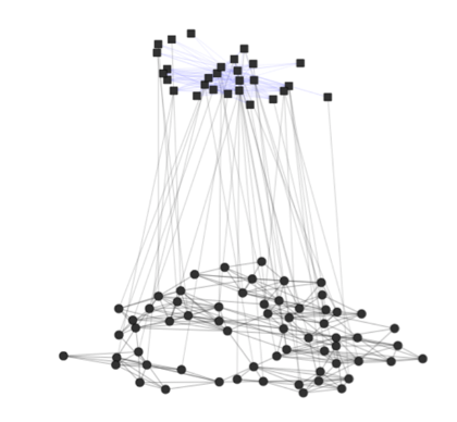
For multilevel structures, we tend to collect the data in different matrices representing the variation of ties within and between levels. Often, we describe the connection between actors as an adjacency matrix and the relations between levels through incidence matrices. The comfortable combination of these matrices into a common structure would represent the multilevel network that could be highly complex.
Let’s assume that we have a multilevel network with two adjacency matrices, one valued matrix and two incidence matrices between them.
A1: Adjacency Matrix of the level 1
B1: incidence Matrix between level 1 and level
2
A2: Adjacency Matrix of the level 2
B2: incidence Matrix between level 2 and level
3
A3: Valued Matrix of the level 3
Create the data
A1 <- matrix(c(
  0, 1, 0, 0, 1,
  1, 0, 0, 1, 1,
  0, 0, 0, 1, 1,
  0, 1, 1, 0, 1,
  1, 1, 1, 1, 0
), byrow = TRUE, ncol = 5)

B1 <- matrix(c(
  1, 0, 0,
  1, 1, 0,
  0, 1, 0,
  0, 1, 0,
  0, 1, 1
), byrow = TRUE, ncol = 3)

A2 <- matrix(c(
  0, 1, 1,
  1, 0, 0,
  1, 0, 0
), byrow = TRUE, nrow = 3)

B2 <- matrix(c(
  1, 1, 0, 0,
  0, 0, 1, 0,
  0, 0, 1, 1
), byrow = TRUE, ncol = 4)

A3 <- matrix(c(
  0, 1, 3, 1,
  1, 0, 0, 0,
  3, 0, 0, 5,
  1, 0, 5, 0
), byrow = TRUE, ncol = 4)
We will start with a report of the matrices:
matrix_report(A1)
#> The matrix A might have the following characteristics:
#> --> The vectors of the matrix are `numeric`
#> --> No names assigned to the rows of the matrix
#> --> No names assigned to the columns of the matrix
#> --> Matrix is symmetric (network is undirected)
#> --> The matrix is square, 5 by 5
#>      nodes edges
#> [1,]     5     7
matrix_report(B1)
#> The matrix A might have the following characteristics:
#> --> The vectors of the matrix are `numeric`
#> --> No names assigned to the rows of the matrix
#> --> No names assigned to the columns of the matrix
#> --> The matrix is rectangular, 3 by 5
#>      nodes_rows nodes_columns incidence_lines
#> [1,]          3             5               7
matrix_report(A2)
#> The matrix A might have the following characteristics:
#> --> The vectors of the matrix are `numeric`
#> --> No names assigned to the rows of the matrix
#> --> No names assigned to the columns of the matrix
#> --> Matrix is symmetric (network is undirected)
#> --> The matrix is square, 3 by 3
#>      nodes edges
#> [1,]     3     2
matrix_report(B2)
#> The matrix A might have the following characteristics:
#> --> The vectors of the matrix are `numeric`
#> --> No names assigned to the rows of the matrix
#> --> No names assigned to the columns of the matrix
#> --> The matrix is rectangular, 4 by 3
#>      nodes_rows nodes_columns incidence_lines
#> [1,]          4             3               5
matrix_report(A3)
#> The matrix A might have the following characteristics:
#> --> The vectors of the matrix are `numeric`
#> --> No names assigned to the rows of the matrix
#> --> No names assigned to the columns of the matrix
#> --> Valued matrix
#> --> Matrix is symmetric (network is undirected)
#> --> The matrix is square, 4 by 4
#>      nodes edges
#> [1,]     4    10
What is the density of some of the matrices?
matrices <- list(A1, B1, A2, B2)
gen_density(matrices, multilayer = TRUE)
#> $`Density of matrix [[1]]`
#> [1] 0.7
#>
#> $`Density of matrix [[2]]`
#> [1] 0.4666667
#>
#> $`Density of matrix [[3]]`
#> [1] 0.6666667
#>
#> $`Density of matrix [[4]]`
#> [1] 0.4166667
How about the degree centrality of the entire structure?
multilevel_degree(A1, B1, A2, B2, complete = TRUE)
#>    multilevel bipartiteB1 bipartiteB2 tripartiteB1B2 low_multilevel
#> n1          3           1          NA              1              3
#> n2          5           2          NA              2              5
#> n3          3           1          NA              1              3
#> n4          4           1          NA              1              4
#> n5          6           2          NA              2              6
#> m1          6           2           2              4              4
#> m2          6           4           1              5              5
#> m3          4           1           2              3              3
#> k1          1          NA           1              1              1
#> k2          1          NA           1              1              1
#> k3          2          NA           2              2              2
#> k4          1          NA           1              1              1
#>    meso_multilevel high_multilevel
#> n1               1               1
#> n2               2               2
#> n3               1               1
#> n4               1               1
#> n5               2               2
#> m1               6               4
#> m2               6               5
#> m3               4               3
#> k1               1               1
#> k2               1               1
#> k3               2               2
#> k4               1               1
Besides, we can perform a k-core analysis of one of the levels using the information of an incidence matrix
k_core(A1, B1, multilevel = TRUE)
#> [1] 3 3 3 3 3
This package also allows performing complex census for multilevel networks.
mixed_census(A2, t(B1), B2, quad = TRUE)
#>   000   100   001   010   020   200  11D0  11U0   120   210   220   002  01D1
#>     2     6     1     0     0     2     0     0     4     0     1     1     0
#>  01U1   012   021   022  101N  101P   201   102   202 11D1W 11U1P 11D1P 11U1W
#>     0     0     8     0     3     0     1     3     1     0     0     0     0
#>  121W  121P  21D1  21U1  11D2  11U2   221   122   212   222
#> 11 13 0 0 0 0 3 0 0 0When we are interested in one particular actor, we could perform
different network measures. For example, actor e has
connections with all the other actors in the network. Therefore, we
could estimate some of Ronald Burt’s measures.
# First we will assign names to the matrix
rownames(A1) <- letters[1:nrow(A1)]
colnames(A1) <- letters[1:ncol(A1)]

eb_constraint(A1, ego = "e")
#> $results
#>   term1 term2 term3 constraint normalization
#> e  0.25 0.292 0.101      0.642         0.761
#>
#> $maximum
#>     e
#> 0.766
redundancy(A1, ego = "e")
#> $redundancy
#> [1] 1.5
#>
#> $effective_size
#> [1] 2.5
#>
#> $efficiency
#> [1] 0.625
Also, sometimes we might want to subset a group of actors surrounding an ego.
ego_net(A1, ego = "e")
#>   a b c d
#> a 0 1 0 0
#> b 1 0 0 1
#> c 0 0 0 1
#> d 0 1 1 0This package expand some measures for one-mode networks, such as the
generalized degree centrality. Suppose we consider a valued matrix
A3. If alpha=0 then it would only count the
direct connections. But, adding the tuning parameter
alpha=0.5 would determine the relative importance of the
number of ties compared to tie weights.
gen_degree(A3, digraph = FALSE, weighted = TRUE)
#> [1] 3.872983 1.000000 4.000000 3.464102
Also, we could conduct some exploratory analysis using the normalized degree of an incidence matrix.
gen_degree(B1, bipartite = TRUE, normalized = TRUE)
#> $bipartiteL1
#> [1] 0.3333333 0.6666667 0.3333333 0.3333333 0.6666667
#>
#> $bipartiteL2
#> [1] 0.4 0.8 0.2
This package also implements some analysis of dyads.
# dyad census
dyadic_census(A1)
#>      Mutual Asymmetrics       Nulls
#>           7           0           3

# Katz and Powell reciprocity
kp_reciprocity(A1)
#> [1] 1

# Z test of the number of arcs
z_arctest(A1)
#>     z     p
#> 1.789 0.074
We can also check the triad census assuming conditional uniform distribution considering different types of dyads (U|MAN)
triad_uman(A1)
#>    label OBS   EXP   VAR   STD
#> 1    003   0 0.083 0.076 0.276
#> 2    012   0 0.000 0.000 0.000
#> 3    102   2 1.750 0.688 0.829
#> 4   021D   0 0.000 0.000 0.000
#> 5   021U   0 0.000 0.000 0.000
#> 6   021C   0 0.000 0.000 0.000
#> 7   111D   0 0.000 0.000 0.000
#> 8   111U   0 0.000 0.000 0.000
#> 9   030T   0 0.000 0.000 0.000
#> 10  030C   0 0.000 0.000 0.000
#> 11   201   5 5.250 1.688 1.299
#> 12  120D   0 0.000 0.000 0.000
#> 13  120U   0 0.000 0.000 0.000
#> 14  120C   0 0.000 0.000 0.000
#> 15   210   0 0.000 0.000 0.000
#> 16 300 3 2.917 0.410 0.640Please note that this project is released with a Contributor Code of Conduct. By participating in this project you agree to abide by its terms.
# library(todor)
# todor::todor_package(c("TODO", "FIXME"))