Interface to the Italian National Institute of Statistics (‘ISTAT’) API
istatR provides an interface to the ‘ISTAT’ ‘SDMX’ RESTful
API, allowing users to:
This package is inspired by the Python ‘istatapi’ package by Jacopo Attolini.
# Install from CRAN

install.packages("istatR")

# Install from source
# devtools::install_github("jfulponi/istatR")

# Or install locally
# devtools::install_local("path/to/istatR")library(istatR)
# List all available datasets
datasets <- all_available()
head(datasets)
#> # A tibble: 6 × 4
#> df_id version df_description df_structure_id
#> <chr> <chr> <chr> <chr>
#> 1 101_1015 1.0 Population by marital status DCIS_POPRES1
#> 2 115_333 1.0 Consumer price index DCSP_IPCA
#> ...
# Search for specific datasets
import_datasets <- search_dataset("import")
population_datasets <- search_dataset("population")# Create dataset by ID
ds <- istat_dataset("139_176")
print(ds)
#> ISTAT Dataset
#> -------------
#> ID: 139_176
#> Version: 1.0
#> Description: Foreign trade - imports and exports
#> Structure: DCSC_COMMEST_EPORT
#>
#> Dimensions (7):
#> - FREQ: (all)
#> - MERCE_ATECO_2007: (all)
#> - PAESE_PARTNER: (all)
#> ...# View dimension information
dimensions_info(ds)
#> # A tibble: 7 × 4
#> dimension_id position codelist_id description
#> <chr> <int> <chr> <chr>
#> 1 FREQ 1 CL_FREQ Frequency
#> 2 MERCE_ATECO_2007 2 CL_MERCE_ATECO2007 Product (ATECO 2007)
#> ...
# Get available values for a specific dimension
get_dimension_values(ds, "TIPO_DATO")
#> # A tibble: 4 × 2
#> id name
#> <chr> <chr>
#> 1 ISAV Imports - value
#> 2 ESAV Exports - value
#> 3 ISAQ Imports - quantity
#> 4 ESAQ Exports - quantity
# Get all available values
available <- get_available_values(ds)
available$FREQ# Set filters
ds <- set_filters(ds,
FREQ = "M",
TIPO_DATO = c("ISAV", "ESAV"), # Multiple values
PAESE_PARTNER = "WORLD"
)
# Retrieve data
data <- get_data(ds)
# Or use time period filters
data <- get_data(ds,
start_period = "2020-01-01",
end_period = "2023-12-31"
)
# Get only the last 12 observations
data <- get_data(ds, last_n_observations = 12)# Combine all steps in one function call
data <- istat_get(
"139_176",
FREQ = "M",
TIPO_DATO = "ISAV",
PAESE_PARTNER = "WORLD",
start_period = "2022-01-01"
)| Function | Description |
|---|---|
all_available() |
List all available ‘ISTAT’ datasets |
search_dataset(keyword) |
Search datasets by keyword in description |
istat_dataset(id) |
Create a dataset object for exploration |
dimensions_info(ds) |
Get information about dataset dimensions |
get_dimension_values(ds, dim) |
Get available values for a dimension |
get_available_values(ds) |
Get all available values for all dimensions |
set_filters(ds, ...) |
Set dimension filters |
reset_filters(ds) |
Reset all filters to default |
get_data(ds) |
Retrieve data with current filters |
istat_get(id, ...) |
Quick retrieval combining all steps |
istat_timeout(seconds) |
Get or set the API timeout |
Note: The ‘ISTAT’ API can be slow to respond, especially when listing all datasets or retrieving large amounts of data. The default timeout is set to 300 seconds (5 minutes) to accommodate this.
If you encounter timeout errors, you can increase the timeout:
# Check current timeout
istat_timeout()
#> [1] 300

# Increase timeout to 10 minutes
istat_timeout(600)

# Or even longer for very large queries
istat_timeout(900) # 15 minutesThis package uses the ‘ISTAT’ ‘SDMX’ REST API: - Base URL:
https://esploradati.istat.it/SDMXWS/rest - Agency ID:
IT1
See the API documentation for more details.
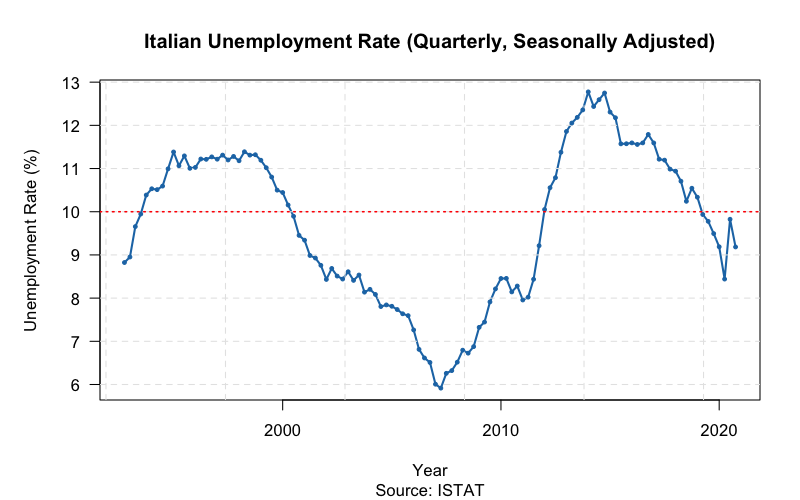
Here’s a complete example that retrieves Italian unemployment rate data and creates a visualization using base R graphics:
library(istatR)

# Search for unemployment datasets
unemp_datasets <- search_dataset("unemployment")
head(unemp_datasets)

# Get quarterly unemployment rate data (seasonally adjusted)
ds <- istat_dataset("151_1178")
ds <- set_filters(ds,
  FREQ = "Q",           # Quarterly data
  REF_AREA = "IT",      # Italy
  DATA_TYPE = "UNEM_R", # Unemployment rate
  SEX = "9",            # Total (both sexes)
  AGE = "Y_GE15"        # 15 years and over
)

unemp_data <- get_data(ds)

# Remove duplicates (different editions) and sort
unemp_data <- unemp_data[!duplicated(unemp_data$TIME_PERIOD), ]
unemp_data <- unemp_data[order(unemp_data$TIME_PERIOD), ]

# Create the plot
par(mar = c(5, 5, 4, 2))
plot(
  unemp_data$TIME_PERIOD,
  unemp_data$OBS_VALUE,
  type = "l",
  lwd = 2,
  col = "#1f77b4",
  xlab = "Year",
  ylab = "Unemployment Rate (%)",
  main = "Italian Unemployment Rate (Quarterly, Seasonally Adjusted)",
  sub = "Source: ISTAT",
  las = 1,
  cex.main = 1.2
)
grid(col = "gray90", lty = 2)

# Add points for emphasis
points(unemp_data$TIME_PERIOD, unemp_data$OBS_VALUE,
       pch = 19, col = "#1f77b4", cex = 0.5)

# Add horizontal reference line at 10%
abline(h = 10, col = "red", lty = 3, lwd = 1.5)
This produces a time series plot showing the evolution of Italian unemployment from 1992 to 2020:
Note: The ‘ISTAT’ API can occasionally be slow or
temporarily unavailable. If you experience connection issues, try again
later or increase the timeout with istat_timeout(600).
Apache License 2.0