 ])
]) The vegan package includes several functions for adding
features to ordination plots: ordiarrows(),
ordiellipse(), ordihull(),
ordispider() and ordisurf(). This package adds
these same features to ordination plots made with ggplot2.
In addition, gg_ordibubble() sizes points relative to the
value of an environmental variable.
The functions are written so that features from each can be combined in customized ordination plots.
The functions ord_labels() and
scale_arrow() (used to ensure vector arrows fit within a
plot) are exported to make it easier to generate custom ordination
plots.
You can install the development version of ggordiplots from GitHub with:
# install.packages("devtools")
devtools::install_github("jfq3/ggordiplots")
You can install the latest release from CRAN with:
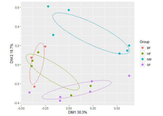
install.packages("ggordiplots")Plot an ordination with ellipses around treatment group centroids (at
distances of one standard deviation) with
gg_ordiplot().
library(ggordiplots)
#> Loading required package: ggplot2
#> Loading required package: vegan
#> Loading required package: permute
#> Loading required package: lattice
#> This is vegan 2.6-4
#> Loading required package: glue
data("dune")
data("dune.env")
dune_bray <- vegdist(dune, method = "bray")
ord <- cmdscale(dune_bray, k = (nrow(dune) - 1), eig = TRUE, add = TRUE)
#> Warning in cmdscale(dune_bray, k = (nrow(dune) - 1), eig = TRUE, add = TRUE):
#> only 18 of the first 19 eigenvalues are > 0
plt1 <- gg_ordiplot(ord, groups = dune.env$Management, plot = FALSE)
plt1 is list with items named:
names(plt1)
#> [1] "df_ord"      "df_mean.ord" "df_ellipse"  "df_hull"     "df_spiders"
#> [6] "plot"
The first 5 items are data frames for making plots. The last item is a ggplot:
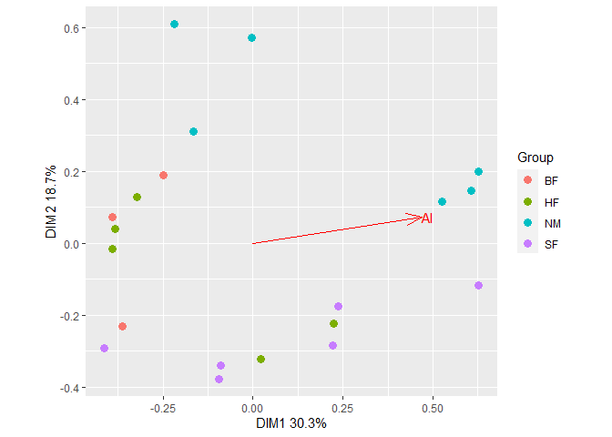
plt1$plot Fit a vector of Al concentrations to the ordination with
gg_envfit().
Al <- as.data.frame(dune.env$A1)
colnames(Al) <- "Al"
plt2 <- gg_envfit(ord, env = Al, groups = dune.env$Management, plot = FALSE)
plt2$plot
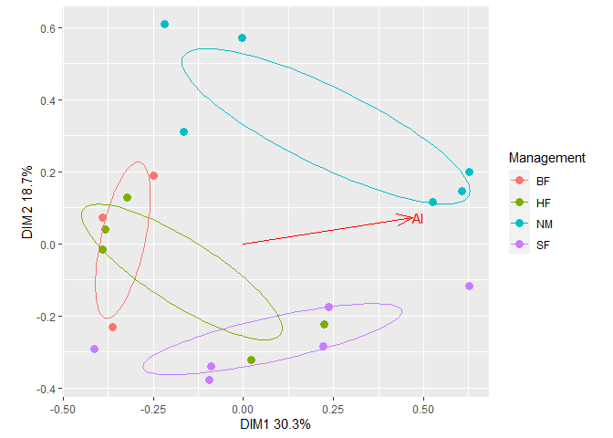
Add ellipses from the first plot to the second plot. The resulting plot
can be further customized using usual
 ggplot2 methods. For
example, change the legend title.
plt2$plot +
  geom_path(data = plt1$df_ellipse, aes(x=x, y=y, color=Group)) +
  guides(color=guide_legend(title="Management")) # Change legend title