

{ggindex} marks selected points of a ggplot2 plot with
numbered markers and explains the numbers in a legend, as on an
annotated map.
Install the released version of {ggindex} from CRAN
with:
install.packages("ggindex")You can install the development version of {ggindex}
from GitHub with:
# install.packages("pak")
pak::pak("discindo/ggindex")Map info to the description that goes in the legend. The
entries are numbered in the order they appear in the data; map
label to choose the numbers yourself.
library(ggplot2)
library(ggindex)

sites <- data.frame(
  x = c(6, 7, 8, 9, 10),
  y = c(6, 9, 7, 10, 8),
  name = c("Library", "Main hall", "Sports centre", "Cafeteria", "Car park")
)

ggplot(sites, aes(x, y, info = name)) +
  geom_focus() +
  theme_minimal()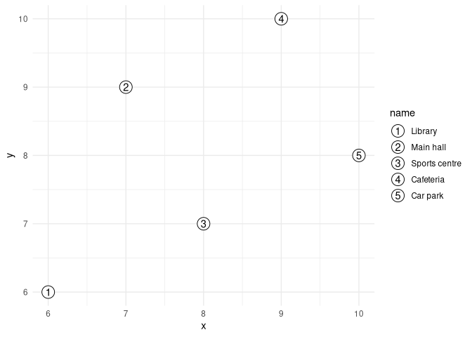
geom_sf_focus() does the same on maps made with the sf
package:
nc <- sf::st_read(system.file("shape/nc.shp", package = "sf"), quiet = TRUE)
nc <- sf::st_transform(nc, 32119)
nc_large <- nc[nc$AREA > 0.2, ]

ggplot(nc) +
  geom_sf(fill = "grey90", colour = "white") +
  geom_sf_focus(aes(info = NAME), data = nc_large) +
  scale_info_discrete("Largest counties") +
  theme_void()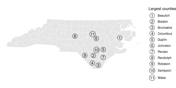
Map focus to number only some observations, and draw the
rest with geom_point(). The markers take the standard
colour, fill, shape and
size aesthetics, so regular ggplot2 scales apply. Here the
most efficient car of each cylinder class is numbered by its overall
rank and filled by class:
cars <- mtcars
cars$model <- rownames(cars)
cars$rank <- rank(-cars$mpg, ties.method = "first")
cars$best <- cars$mpg == ave(cars$mpg, cars$cyl, FUN = max)

ggplot(cars, aes(wt, mpg)) +
  geom_point(colour = "grey60") +
  geom_focus(aes(label = rank, focus = best, info = model, fill = factor(cyl))) +
  scale_fill_brewer("Cylinders", palette = "Set2") +
  scale_info_discrete("Best in class") +
  labs(x = "Weight (1000 lbs)", y = "Miles per gallon") +
  theme_minimal()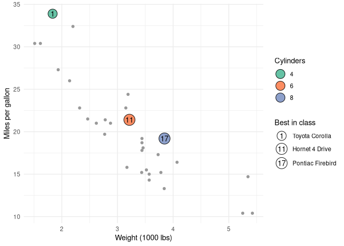
Map label, focus and info in
geom_focus() when the plot has other layers: layers inherit
the mapping of ggplot(), and their observations would also
appear in the legend.