Help for package Ternary

Version:

2.3.4

Title:

Create Ternary and Holdridge Plots

Description:

Plots ternary diagrams (simplex plots / Gibbs triangles) and Holdridge life zone plots <doi:10.1126/science.105.2727.367> using the standard graphics functions. Allows custom annotation, interpolating, contouring and scaling of plotting region. Includes a 'Shiny' user interface for point-and-click ternary plotting. An alternative to 'ggtern', which uses the 'ggplot2' family of plotting functions.

URL:

https://ms609.github.io/Ternary/, https://github.com/ms609/Ternary/

BugReports:

https://github.com/ms609/Ternary/issues/

License:

GPL-2 | GPL-3 [expanded from: GPL (≥ 2)]

Language:

en-GB

Depends:

R (≥ 3.6.0)

Imports:

PlotTools (≥ 0.2.0), RcppHungarian, shiny, sp,

Suggests:

colourpicker, knitr, readxl, rmarkdown, shinyjs, spelling, testthat (≥ 3.0), vdiffr,

Config/Needs/check:

rcmdcheck

Config/Needs/coverage:

covr

Config/Needs/memcheck:

devtools, rcmdcheck

Config/Needs/metadata:

codemeta

Config/Needs/revdeps:

revdepcheck

Config/Needs/website:

pkgdown

Config/testthat/edition:

Config/testthat/parallel:

false

LazyData:

true

VignetteBuilder:

knitr

Encoding:

UTF-8

RoxygenNote:

7.3.2

NeedsCompilation:

Packaged:

2025-05-07 12:48:46 UTC; pjjg18

Author:

Martin R. Smith

[aut, cre, cph], Lilian Sanselme [ctb]

Maintainer:

Martin R. Smith <martin.smith@durham.ac.uk>

Repository:

CRAN

Date/Publication:

2025-05-07 13:30:02 UTC

The 'Ternary' package allows the creation of ternary plots (a.k.a. ternary graphs / simplex plots / Gibbs triangles / de Finetti diagrams) using the familiar functions of the default 'graphics' package.

Description

For simple use cases, generate ternary plots using the point-and-click Shiny app:

Details

install.packages('Ternary')
Ternary::TernaryApp()

For greater control over your plots, use the R command line; for usage instructions, consult the guidance article online or by typing vignette('Ternary', 'Ternary') at the R console.

Author(s)

Maintainer: Martin R. Smith martin.smith@durham.ac.uk (ORCID) [copyright holder]

Other contributors:

Lilian Sanselme [contributor]

Set plotting region

Description

Sets the region of the ternary plot being drawn. Usually called from within TernaryPlot(); everyday users are unlikely to need to call this function directly.

Usage

.SetRegion(region, prettify = NA_integer_, set = TRUE)

Arguments

region

(optional) Named list of length two specifying the the minimum and maximum values of each ternary axis to be drawn (e.g. ⁠list(min = c(40, 0, 0), max = c(100, 60, 60)⁠); or a set of coordinates in a format accepted by TernaryPoints(). The plotted region will correspond to the smallest equilateral triangle that encompasses the specified ranges or coordinates.

prettify

If numeric, the plotting region will be expanded to allow grid lines to be produced with pretty(n = prettify). If NA, the smallest region encompassing region will be used.

set

Logical specifying whether to set options(ternRegion = region)

Value

.SetRegion() returns the value of options(ternRegion = region) if set == TRUE, or the region, otherwise..

Author(s)

Martin R. Smith (martin.smith@durham.ac.uk)

Examples

# XY Coordinates under original plotting region
TernaryToXY(c(1, 2, 3))
previous <- .SetRegion(rbind(min = c(20, 20, 20), max = c(60, 60, 60)))

# New region options set
getOption("ternRegion")

# Coordinates under new plotting region
TernaryToXY(c(1, 2, 3))

# Restore previous setting
options(previous)
getOption("ternRegion")

Add elements to ternary or Holdridge plot

Description

Plot shapes onto a ternary diagram created with TernaryPlot(), or a Holdridge plot created with HoldridgePlot().

Usage

AddToTernary(PlottingFunction, coordinates, ...)

TernaryArrows(fromCoordinates, toCoordinates = fromCoordinates, ...)

TernaryLines(coordinates, ...)

TernaryPoints(coordinates, ...)

TernaryPolygon(coordinates, ...)

TernarySegments(fromCoordinates, toCoordinates = fromCoordinates, ...)

TernaryText(coordinates, ...)

JoinTheDots(coordinates, ...)

AddToHoldridge(PlottingFunction, pet, prec, ...)

HoldridgeArrows(fromCoordinates, toCoordinates = fromCoordinates, ...)

HoldridgeLines(pet, prec, ...)

HoldridgePoints(pet, prec, ...)

HoldridgePolygon(pet, prec, ...)

HoldridgeText(pet, prec, ...)

Arguments

PlottingFunction

Function to add data to a plot; perhaps one of points, lines or text.

coordinates

A list, matrix, data.frame or vector in which each element (or row) specifies the three coordinates of a point in ternary space.

...

Additional parameters to pass to PlottingFunction(). If using TernaryText(), this will likely include the parameter labels, to specify the text to plot. Other useful graphical parameters include srt to rotate text.

fromCoordinates, toCoordinates

For TernaryArrows(), coordinates at which arrows should begin and end; cf. x0, y0, x1 and y1 in arrows. Recycled as necessary.

pet, prec

Numeric vectors giving potential evapotranspiration ratio and annual precipitation (in mm).

Functions

TernaryArrows(): Add arrows
TernaryLines(): Add lines
TernaryPoints(): Add points
TernaryPolygon(): Add polygons
TernarySegments(): Add segments
TernaryText(): Add text
JoinTheDots(): Add points, joined by lines
HoldridgeArrows(): Add arrows to Holdridge plot
HoldridgeLines(): Add lines to Holdridge plot
HoldridgePoints(): Add points to Holdridge plot
HoldridgePolygon(): Add polygons to Holdridge plot
HoldridgeText(): Add text to Holdridge plot

Author(s)

Martin R. Smith (martin.smith@durham.ac.uk)

Examples

# Data to plot
coords <- list(
  A = c(1, 0, 2),
  B = c(1, 1, 1),
  C = c(1.5, 1.5, 0),
  D = c(0.5, 1.5, 1)
)

# Set up plot
oPar <- par(mar = rep(0, 4), xpd = NA) # reduce margins and write in them
TernaryPlot()

# Add elements to ternary diagram
AddToTernary(lines, coords, col = "darkgreen", lty = "dotted", lwd = 3)
TernaryLines(coords, col = "darkgreen")
TernaryArrows(coords[1], coords[2:4], col = "orange", length = 0.2, lwd = 1)
TernaryText(coords, cex = 0.8, col = "red", font = 2)
seeThruBlue <- rgb(0, 0.2, 1, alpha = 0.8)
TernaryPoints(coords, pch = 1, cex = 2, col = seeThruBlue)
AddToTernary(graphics::points, coords, pch = 1, cex = 3)

# An equivalent syntax applies to Holdridge plots:
HoldridgePlot()
pet <- c(0.8, 2, 0.42)
prec <- c(250, 400, 1337)
HoldridgeText(pet, prec, c("A", "B", "C"))
AddToHoldridge(graphics::points, pet, prec, cex = 3)

# Restore original plotting parameters
par(oPar)

Annotate points on a ternary plot

Description

Annotate() identifies and label individual points on a ternary diagram in the plot margins.

Usage

Annotate(
  coordinates,
  labels,
  side,
  outset = 0.16,
  line.col = col,
  lty = par("lty"),
  lwd = par("lwd"),
  col = par("col"),
  font = par("font"),
  offset = 0.5,
  ...
)

Arguments

coordinates

A list, matrix, data.frame or vector in which each element (or row) specifies the three coordinates of a point in ternary space.

labels

Character vector specifying text with which to annotate each entry in coordinates.

side

Optional vector specifying which side of the ternary plot each point should be labelled on, using the notation ⁠"a", "b", "c"⁠ or ⁠1, 2, 3⁠. Entries of "n" or 0 will not be annotated (but still require an entry in labels). Entries of NA will be allocated a side automatically, based on the midpoint of coordinates.

outset

Numeric specifying distance from plot margins to labels.

line.col, lty, lwd

parameters to segments().

col, font, offset

parameters to text().

...

Further parameters to text() and segments().

Author(s)

Martin R. Smith (martin.smith@durham.ac.uk)

Examples

# Load some data
data("Seatbelts")
seats <- c("drivers", "front", "rear")
seat <- Seatbelts[month.abb %in% "Oct", seats]
law <- Seatbelts[month.abb %in% "Oct", "law"]

# Set up plot
oPar <- par(mar = c(2, 0, 0, 0))
TernaryPlot(alab = seats[1], blab = seats[2], clab = seats[3])
TernaryPoints(seat, cex = 0.8, col = 2 + law)

# Annotate points by year
Annotate(seat, labels = 1969:1984, col = 2 + law)

# Restore original graphical parameters
par(oPar)

Colour ternary plot

Description

Colour a ternary plot according to the output of a function.

Usage

ColourTernary(
  values,
  spectrum = hcl.colors(256L, palette = "viridis", alpha = 0.6),
  resolution = sqrt(ncol(values)),
  direction = getOption("ternDirection", 1L),
  legend,
  ...
)

ColorTernary(
  values,
  spectrum = hcl.colors(256L, palette = "viridis", alpha = 0.6),
  resolution = sqrt(ncol(values)),
  direction = getOption("ternDirection", 1L),
  legend,
  ...
)

Arguments

values

Numeric matrix, possibly created using TernaryPointValues(), with four named rows: x, y, Cartesian coordinates of each triangle centre; z, value associated with that coordinate; down, triangle direction: 0 = point upwards; 1 = point downwards.

spectrum

Vector of colours to use as a spectrum, or NULL to use values["z", ].

resolution

The number of triangles whose base should lie on the longest axis of the triangle. Higher numbers will result in smaller subdivisions and smoother colour gradients, but at a computational cost.

direction

(optional) Integer specifying the direction that the current ternary plot should point: 1, up; 2, right; 3, down; 4, left.

legend

Character vector specifying annotations for colour scale. If not provided, no colour legend is displayed. Specify TRUE to generate automatically, or a single integer to generate legend annotations.

...

Further arguments to SpectrumLegend().

Value

ColourTernary() is called for its side effect – colouring a ternary plot according to values. It invisibly returns NULL.

Author(s)

Martin R. Smith (martin.smith@durham.ac.uk)

Examples

# Depict a function across a ternary plot with colour and contours

TernaryPlot(alab = "a", blab = "b", clab = "c") # Blank plot

FunctionToContour <- function (a, b, c) {
  a - c + (4 * a * b) + (27 * a * b * c)
}

# Evaluate function
values <- TernaryPointValues(FunctionToContour, resolution = 24L)

# Use the value of the function to determine the brightness of the plot
ColourTernary(
  values,
  x = "topleft",
  bty = "n", # No box
  legend = signif(seq(max(values), min(values), length.out = 4), 3)
)

# Overlay contours
TernaryContour(FunctionToContour, resolution = 36L)

# Directly specify the colour with the output of a function

# Create a function that returns a vector of rgb strings:
rgbWhite <- function (r, g, b) {
  highest <- apply(rbind(r, g, b), 2L, max)
  rgb(r/highest, g/highest, b/highest)
}

TernaryPlot()
values <- TernaryPointValues(rgbWhite, resolution = 20)
ColourTernary(values, spectrum = NULL)

Convert a point in evapotranspiration-precipitation space to an appropriate cross-blended hypsometric colour

Description

Used to colour HoldridgeHexagons(), and may also be used to aid the interpretation of PET + precipitation data in any graphical context.

Usage

HoldridgeHypsometricCol(pet, prec, opacity = NA)

Arguments

pet, prec

Numeric vectors giving potential evapotranspiration ratio and annual precipitation (in mm).

opacity

Opacity level to be converted to the final two characters of an RGBA hexadecimal colour definition, e.g. ⁠#000000FF⁠. Specify a character string, which will be interpreted as a hexadecimal alpha value and appended to the six RGB hexadecimal digits; a numeric in the range 0 (transparent) to 1 (opaque); or NA, to return only the six RGB digits.

Value

Character vector listing RGB or (if opacity != NA) RGBA values corresponding to each PET-precipitation value pair.

Author(s)

Martin R. Smith (martin.smith@durham.ac.uk)

References

Palette derived from the hypsometric colour scheme presented at Shaded Relief.

Examples

HoldridgePlot(hex.col = HoldridgeHypsometricCol)
VeryTransparent <- function(...) HoldridgeHypsometricCol(..., opacity = 0.3)
HoldridgePlot(hex.col = VeryTransparent)
pet <- holdridge$PET
prec <- holdridge$Precipitation
ptCol <- HoldridgeHypsometricCol(pet, prec)
HoldridgePoints(pet, prec, pch = 21, bg = ptCol)

Plot life zones on a Holdridge plot

Description

HoldridgePlot() creates a blank triangular plot, as proposed by Holdridge (1947, 1967), onto which potential evapotranspiration (PET) ratio and annual precipitation data can be plotted (using the AddToHoldridge() family of functions) in order to interpret climatic life zones.

Usage

HoldridgePlot(
  atip = NULL,
  btip = NULL,
  ctip = NULL,
  alab = "Potential evapotranspiration ratio",
  blab = "Annual precipitation / mm",
  clab = "Humidity province",
  lab.offset = 0.22,
  lab.col = c("#D81B60", "#1E88E5", "#111111"),
  xlim = NULL,
  ylim = NULL,
  region = NULL,
  lab.cex = 1,
  lab.font = 0,
  tip.cex = lab.cex,
  tip.font = 2,
  tip.col = "black",
  isometric = TRUE,
  atip.rotate = NULL,
  btip.rotate = NULL,
  ctip.rotate = NULL,
  atip.pos = NULL,
  btip.pos = NULL,
  ctip.pos = NULL,
  padding = 0.16,
  col = NA,
  panel.first = NULL,
  panel.last = NULL,
  grid.lines = 8,
  grid.col = c(NA, "#1E88E5", "#D81B60"),
  grid.lty = "solid",
  grid.lwd = par("lwd"),
  grid.minor.lines = 0,
  grid.minor.col = "lightgrey",
  grid.minor.lty = "solid",
  grid.minor.lwd = par("lwd"),
  hex.border = "#888888",
  hex.col = HoldridgeHypsometricCol,
  hex.lty = "solid",
  hex.lwd = par("lwd"),
  hex.cex = 0.5,
  hex.labels = NULL,
  hex.font = NULL,
  hex.text.col = "black",
  axis.cex = 0.8,
  axis.col = c(grid.col[2], grid.col[3], NA),
  axis.font = par("font"),
  axis.labels = TRUE,
  axis.lty = "solid",
  axis.lwd = 1,
  axis.rotate = TRUE,
  axis.pos = NULL,
  axis.tick = TRUE,
  ticks.lwd = axis.lwd,
  ticks.length = 0.025,
  ticks.col = grid.col,
  ...
)

HoldridgeBelts(
  grid.col = "#004D40",
  grid.lty = "dotted",
  grid.lwd = par("lwd")
)

HoldridgeHexagons(
  border = "#004D40",
  hex.col = HoldridgeHypsometricCol,
  lty = "dotted",
  lwd = par("lwd"),
  labels = NULL,
  cex = 1,
  text.col = NULL,
  font = NULL
)

Arguments

atip, btip, ctip

Character string specifying text to title corners, proceeding clockwise from the corner specified in point (default: top).

alab, blab, clab

Character string specifying text with which to label the corresponding sides of the triangle. Left or right-pointing arrows are produced by typing ⁠\\U2190⁠ or ⁠\\U2192⁠, or using expression('value' %->% '').

lab.offset

Numeric specifying distance between midpoint of axis label and the axis. The default value is given in the 'Usage' section; a value of 0 will position the axis label directly on the axis. Increase padding if labels are being clipped. Use a vector of length three to specify a different offset for each label.

lab.col

Character vector specifying colours for axis labels. Use a vector of length three to specify a different colour for each label.

xlim, ylim

Numeric vectors of length two specifying the minimum and maximum x and y limits of the plotted area, to which padding will be added. The default is to display the complete height or width of the plot. Allows cropping to magnified region of the plot. (See vignette for diagram.) May be overridden if isometric = TRUE; see documentation of isometric parameter.

region

lab.cex, tip.cex

Numeric specifying character expansion (font size) for axis labels. Use a vector of length three to specify a different value for each direction.

lab.font, tip.font

Numeric specifying font style (Roman, bold, italic, bold-italic) for axis titles. Use a vector of length three to set a different font for each direction.

isometric

Logical specifying whether to enforce an equilateral shape for the ternary plot. If only one of xlim and ylim is set, the other will be calculated to maintain an equilateral plot. If both xlim and ylim are set, but have different ranges, then the limit with the smaller range will be scaled until its range matches that of the other limit.

atip.rotate, btip.rotate, ctip.rotate

Integer specifying number of degrees to rotate label of rightmost apex.

atip.pos, btip.pos, ctip.pos

Integer specifying positioning of labels, iff the corresponding xtip.rotate parameter is set.

padding

Numeric specifying size of internal margin of the plot; increase if axis labels are being clipped.

col

The colour for filling the plot; see polygon.

panel.first

An expression to be evaluated after the plot axes are set up but before any plotting takes place. This can be useful for drawing backgrounds, e.g. with ColourTernary() or HorizontalGrid(). Note that this works by lazy evaluation: passing this argument from other plot methods may well not work since it may be evaluated too early.

panel.last

An expression to be evaluated after plotting has taken place but before the axes and box are added. See the comments about panel.first.

grid.lines

Integer specifying the number of grid lines to plot. If axis.labels = TRUE, this will be used as a hint to pretty().

grid.col, grid.minor.col

Colours to draw the grid lines. Use a vector of length three to set different values for each direction.

grid.lty, grid.minor.lty

Character or integer vector; line type of the grid lines. Use a vector of length three to set different values for each direction.

grid.lwd, grid.minor.lwd

Non-negative numeric giving line width of the grid lines. Use a vector of length three to set different values for each direction.

grid.minor.lines

Integer specifying the number of minor (unlabelled) grid lines to plot between each major pair.

hex.border, hex.lty, hex.lwd

Parameters to pass to HoldridgeHexagons(). Set to NA to suppress hexagons.

hex.col

Fill colour for hexagons. Provide a vector specifying a colour for each hexagon in turn, reading from left to right and top to bottom, or a function that accepts two arguments, numerics pet and prec, and returns a colour in a format accepted by polygon().

hex.cex, hex.font, hex.text.col

Parameters passed to text() to plot hex.labels.

hex.labels

38-element character vector specifying label for each hexagonal class, from top left to bottom right.

axis.cex

Numeric specifying character expansion (font size) for axis labels. Use a vector of length three to set a different value for each direction.

axis.col, ticks.col, tip.col

Colours for the axis line, tick marks and tip labels respectively. Use a vector of length three to set a different value for each direction. axis.col = NULL means to use par('fg'), possibly specified inline, and ticks.col = NULL means to use whatever colour axis.col resolved to.

axis.font

Font for text. Defaults to par('font').

axis.labels

This can either be a logical value specifying whether (numerical) annotations are to be made at the tickmarks, or a character or expression vector of labels to be placed at the tick points, or a list of length three, with each entry specifying labels to be placed on each axis in turn.

axis.lty

Line type for both the axis line and tick marks. Use a vector of length three to set a different value for each direction.

axis.lwd, ticks.lwd

Line width for the axis line and tick marks. Zero or negative values will suppress the line or ticks. Use a vector of length three to set different values for each axis.

axis.rotate

Logical specifying whether to rotate axis labels to parallel grid lines, or numeric specifying custom rotation for each axis, to be passed as srt parameter to text(). Expand margins or set par(xpd = NA) if labels are clipped.

axis.pos

Vector of length one or three specifying position of axis labels, to be passed as pos parameter to text(); populated automatically if NULL (the default).

axis.tick

Logical specifying whether to mark the axes with tick marks.

ticks.length

Numeric specifying distance that ticks should extend beyond the plot margin. Also affects position of axis labels, which are plotted at the end of each tick. Use a vector of length three to set a different length for each direction.

...

Additional parameters to plot.

border

Colour to use for hexagon borders.

lty, lwd, cex, font

Graphical parameters specifying properties of hexagons to be plotted.

labels

Vector specifying labels for life zone hexagons to be plotted. Suggested values: holdridgeClassesUp, holdridgeLifeZonesUp.

text.col

Colour of text to be printed in hexagons.

Details

HoldridgePoints(), HoldridgeText() and related functions allow data points to be added to an existing plot; AddToHoldridge() allows plotting using any of the standard plotting functions.

HoldridgeBelts() and HoldridgeHexagons() plot interpretative lines and hexagons allowing plotted data to be linked to interpreted climate settings.

Please cite Tsakalos et al. (2023) when using this function.

Author(s)

Martin R. Smith (martin.smith@durham.ac.uk)

References

Holdridge (1947), "Determination of world plant formations from simple climatic data", Science 105:367–368. doi:10.1126/science.105.2727.367

Holdridge (1967), Life zone ecology. Tropical Science Center, San José

Tsakalos, Smith, Luebert & Mucina (2023). "climenv: Download, extract and visualise climatic and elevation data.", Journal of Vegetation Science 6:e13215. doi:10.1111/jvs.13215

Examples

data(holdridgeLifeZonesUp, package = "Ternary")
HoldridgePlot(hex.labels = holdridgeLifeZonesUp)
HoldridgeBelts()

Convert user-specified ternary coordinates into X and Y coordinates

Description

Accepts various formats of input data; extracts ternary coordinates and converts to X and Y coordinates.

Usage

HoldridgeToXY(pet, prec)

CoordinatesToXY(coordinates)

Arguments

pet, prec

Numeric vectors giving potential evapotranspiration ratio and annual precipitation (in mm).

coordinates

A list, matrix, data.frame or vector in which each element (or row) specifies the three coordinates of a point in ternary space.

Value

CoordinatesToXY() returns an array of two rows, corresponding to the X and Y coordinates of coordinates.

Functions

HoldridgeToXY(): Convert from Holdridge coordinates

Author(s)

Martin R. Smith (martin.smith@durham.ac.uk)

Is a point in the plotting area?

Description

Evaluate whether a given set of coordinates lie outwith the boundaries of a plotted ternary diagram.

Usage

OutsidePlot(x, y, tolerance = 0)

Arguments

x, y

Vectors of x and y coordinates of points.

tolerance

Consider points this close to the edge of the plot to be inside. Set to negative values to count points that are just outside the plot as inside, and to positive values to count points that are just inside the margins as outside. Maximum positive value: 1/3.

Value

OutsidePlot() returns a logical vector specifying whether each pair of x and y coordinates corresponds to a point outside the plotted ternary diagram.

Author(s)

Martin R. Smith (martin.smith@durham.ac.uk)

Examples


TernaryPlot()
points(0.5, 0.5, col = "darkgreen")
OutsidePlot(0.5, 0.5)

points(0.1, 0.5, col = "red")
OutsidePlot(0.1, 0.5)

OutsidePlot(c(0.5, 0.1), 0.5)

Polygon geometry

Description

Geometry functions for irregular polygons.

Usage

PolygonArea(x, y = NULL, positive = TRUE)

PolygonCentre(x, y = NULL)

PolygonCenter(x, y = NULL)

GrowPolygon(x, y = NULL, buffer = 0)

Arguments

x, y

Vectors containing the coordinates of the vertices of the polygon.

positive

If vertices are specified in an anticlockwise direction, the polygon will be treated as a hole, with a negative area, unless positive is set to TRUE. Vertices specified in a clockwise sequence always yield a positive area.

buffer

Numeric specifying distance by which to grow polygon.

Value

PolygonArea() returns the area of the specified polygon.

PolygonCentre() returns a single-row matrix containing the x and y coordinates of the geometric centre of the polygon.

GrowPolygon() returns coordinates of the vertices of polygon after moving each vertex buffer away from the polygon's centre.

Functions

PolygonArea(): Calculate the area of an irregular polygon
PolygonCentre(): Locate the centre of a polygon
GrowPolygon(): Enlarge a polygon in all directions

Author(s)

Martin R. Smith (martin.smith@durham.ac.uk)

Examples

x <- c(-3, -1, 6, 3, -4)
y <- c(-2, 4, 1, 10, 9)
plot(x, y, frame.plot = FALSE)
polygon(x, y)
PolygonArea(x, y)
points(PolygonCentre(x, y), pch = 3, cex = 2)
polygon(GrowPolygon(x, y, 1), border = "darkgreen",
        xpd = NA # Allow drawing beyond plot border
       )

# Negative values shrink the polygon
polygon(GrowPolygon(x, y, -1), border = "red")

Reflected equivalents of points outside the ternary plot

Description

To avoid edge effects, it may be desirable to add the value of a point within a ternary plot with the value of its 'reflection' across the nearest axis or corner.

Usage

ReflectedEquivalents(x, y, direction = getOption("ternDirection", 1L))

Arguments

x, y

Vectors of x and y coordinates of points.

direction

(optional) Integer specifying the direction that the current ternary plot should point: 1, up; 2, right; 3, down; 4, left.

Value

ReflectedEquivalents() returns a list of the x, y coordinates of the points produced if the given point is reflected across each of the edges or corners.

Examples

TernaryPlot(axis.labels = FALSE, point = 4)

xy <- cbind(
  TernaryCoords(0.9, 0.08, 0.02),
  TernaryCoords(0.15, 0.8, 0.05),
  TernaryCoords(0.05, 0.1, 0.85)
)
x <- xy[1, ]
y <- xy[2, ]

points(x, y, col = "red", pch = 1:3)
ref <- ReflectedEquivalents(x, y)
points(ref[[1]][, 1], ref[[1]][, 2], col = "blue", pch = 1)
points(ref[[2]][, 1], ref[[2]][, 2], col = "green", pch = 2)
points(ref[[3]][, 1], ref[[3]][, 2], col = "orange", pch = 3)

Graphical user interface for creating ternary plots

Description

TernaryApp() launches a 'Shiny' application for the construction of ternary plots. The 'app' allows data to be loaded and plotted, and provides code to reproduce the plot in R should more sophisticated plotting functions be desired.

Usage

TernaryApp()

Details

Load data

The 'Load data' input tab allows for the upload of datasets. Data can be read from csv files, .txt files created with write.table(), or (if the 'readxl' package is installed) Excel spreadsheets.

Data should be provided as three columns, corresponding to the three axes of the ternary plot. Colours or point styles may be specified in columns four to six to allow different categories of point to be plotted distinctly. Example datasets are installed at system.file("TernaryApp", package = "Ternary").

Axes are automatically labelled using column names, if present; these can be edited manually on this tab.

Plot display

Allows the orientation, colour and configuration of the plot and its axes to be adjusted,

Grids

Adjust the number, spacing and styling of major and minor grid lines.

Labels

Configure the colour, position and size of tip and axis labels.

Points

Choose whether to plot points, lines, connected points, or text. Set the style of points and lines.

Exporting plots

A plot can be saved to PDF or as a PNG bitmap at a specified size. Alternatively, R script that will generate the displayed plot can be viewed (using the 'R code' output tab) or downloaded to file.

Author(s)

Martin R. Smith (martin.smith@durham.ac.uk)

References

If you use figures produced with this package in a publication, please cite

Smith, Martin R. (2017). Ternary: An R Package for Creating Ternary Plots. Zenodo, doi: doi:10.5281/zenodo.1068996.

Add contours to a ternary plot

Description

Draws contour lines to depict the value of a function in ternary space.

Usage

TernaryContour(
  Func,
  resolution = 96L,
  direction = getOption("ternDirection", 1L),
  region = getOption("ternRegion", ternRegionDefault),
  within = NULL,
  filled = FALSE,
  legend,
  legend... = list(),
  nlevels = 10,
  levels = pretty(zlim, nlevels),
  zlim,
  color.palette = function(n) hcl.colors(n, palette = "viridis", alpha = 0.6),
  fill.col = color.palette(length(levels) - 1),
  func... = list(),
  ...
)

Arguments

Func

Function that takes three arguments named a, b and c, and returns a numeric vector of length n. a, b and c will each be a vector of length n. Together, they specify the series of coordinates at which the function should be evaluated.

resolution

The number of triangles whose base should lie on the longest axis of the triangle. Higher numbers will result in smaller subdivisions and smoother colour gradients, but at a computational cost.

direction

(optional) Integer specifying the direction that the current ternary plot should point: 1, up; 2, right; 3, down; 4, left.

region

within

List or matrix of x, y coordinates within which contours should be evaluated, in any format supported by xy.coords(x = within). If NULL, defaults to a region slightly smaller than the ternary plot. The ⁠$hull⁠ entry generated by TriangleInHull() may also be used.

filled

Logical; if TRUE, contours will be filled (using .filled.contour().).

legend

legend...

List of additional parameters to send to SpectrumLegend().

nlevels, levels, zlim, ...

parameters to pass to contour().

color.palette

parameters to pass to .filled.contour().

fill.col

Sent as col parameter to .filled.contour(). Computed from color.palette if not specified.

func...

List of additional parameters to send to Func().

Value

TernaryContour() is called for its side effect – adding contours to a Ternary plot according to the value of Func(a, b, c) at each coordinate. It invisibly returns a list containing:

x,y: the Cartesian coordinates of each evaluated point;
z: The value of Func() at each coordinate.

Author(s)

Martin R. Smith (martin.smith@durham.ac.uk)

Examples

FunctionToContour <- function (a, b, c) {
  a - c + (4 * a * b) + (27 * a * b * c)
}

# Set up plot
originalPar <- par(mar = rep(0, 4))
TernaryPlot(alab = "a", blab = "b", clab = "c")
values <- TernaryPointValues(FunctionToContour, resolution = 24L)
ColourTernary(
  values,
  legend = signif(seq(max(values), min(values), length.out = 4), 2),
  bty = "n"
)
TernaryContour(FunctionToContour, resolution = 36L)

# Note that FunctionToContour() is sent vectors of all values of a, b and
# c at which it will be evaluated.
# Instead of
BadMax <- function (a, b, c) {
  max(a, b, c) # Not vectorized
  # Will return the single maximum of ALL a, b and c coordinates
}

# Use
GoodMax <- function (a, b, c) {
  pmax(a, b, c) # Vectorized
  # Will return the maximum of each trio of a, b and c coordinates
}
TernaryPlot(alab = "a", blab = "b", clab = "c")
ColourTernary(TernaryPointValues(GoodMax))
TernaryContour(GoodMax)

# When a vectorized version of a function is not available, you will need to
# apply the function to each combination of a, b and c in turn:
GeneralMax <- function (a, b, c) {
  abc.matrix <- rbind(a, b, c) # Matrix where each column gives an a,b,c trio
  apply(abc.matrix, 2, max)    # Apply non-vectorized function to each trio
  # Returns a vector with the maximum value of a,b,c at each coordinate.
}
TernaryPlot(alab = "a", blab = "b", clab = "c")
# Fill the contour areas, rather than using tiles
TernaryContour(GeneralMax, filled = TRUE,
               legend = c("Max", "...", "Min"),
               legend... = list(bty = "n", xpd = NA), # Tweak legend display
               fill.col =  hcl.colors(14, palette = "viridis", alpha = 0.6))
# Re-draw edges of plot triangle over fill
TernaryPolygon(diag(3))

# Restore plotting parameters
par(originalPar)

Convert ternary coordinates to Cartesian space

Description

Convert coordinates of a point in ternary space, in the format (a, b, c), to x and y coordinates of Cartesian space, which can be sent to standard functions in the 'graphics' package.

Usage

TernaryCoords(
  abc,
  b_coord = NULL,
  c_coord = NULL,
  direction = getOption("ternDirection", 1L),
  region = getOption("ternRegion", ternRegionDefault)
)

## S3 method for class 'matrix'
TernaryToXY(
  abc,
  b_coord = NULL,
  c_coord = NULL,
  direction = getOption("ternDirection", 1L),
  region = getOption("ternRegion", ternRegionDefault)
)

## S3 method for class 'numeric'
TernaryToXY(
  abc,
  b_coord = NULL,
  c_coord = NULL,
  direction = getOption("ternDirection", 1L),
  region = getOption("ternRegion", ternRegionDefault)
)

TernaryToXY(
  abc,
  b_coord = NULL,
  c_coord = NULL,
  direction = getOption("ternDirection", 1L),
  region = getOption("ternRegion", ternRegionDefault)
)

Arguments

abc

A vector of length three giving the position on a ternary plot that points in the direction specified by direction (1 = up, 2 = right, 3 = down, 4 = left). c(100, 0, 0) will plot in the direction-most corner; c(0, 100, 0) will plot in the corner clockwise of direction; c(0, 0, 100) will plot in the corner anti-clockwise of direction. Alternatively, the a coordinate can be specified as the first parameter, in which case the b and c coordinates must be specified via b_coord and c_coord. Or, a matrix with three rows, representing in turn the a, b and c coordinates of points.

b_coord

The b coordinate, if abc is a single number.

c_coord

The c coordinate, if abc is a single number.

direction

(optional) Integer specifying the direction that the current ternary plot should point: 1, up; 2, right; 3, down; 4, left.

region

Value

TernaryCoords() returns a vector of length two that converts the coordinates given in abc into Cartesian (x, y) coordinates corresponding to the plot created by the last call of TernaryPlot().

Author(s)

Martin R. Smith (martin.smith@durham.ac.uk)

Examples

TernaryCoords(100, 0, 0)
TernaryCoords(c(0, 100, 0))

coords <- matrix(1:12, nrow = 3)
TernaryToXY(coords)

Add contours of estimated point density to a ternary plot

Description

Use two-dimensional kernel density estimation to plot contours of point density.

Usage

TernaryDensityContour(
  coordinates,
  bandwidth,
  resolution = 25L,
  tolerance = -0.2/resolution,
  edgeCorrection = TRUE,
  direction = getOption("ternDirection", 1L),
  filled = FALSE,
  nlevels = 10,
  levels = pretty(zlim, nlevels),
  zlim,
  color.palette = function(n) hcl.colors(n, palette = "viridis", alpha = 0.6),
  fill.col = color.palette(length(levels) - 1),
  ...
)

Arguments

coordinates

A list, matrix, data.frame or vector in which each element (or row) specifies the three coordinates of a point in ternary space.

bandwidth

Vector of bandwidths for x and y directions. Defaults to normal reference bandwidth (see MASS::bandwidth.nrd). A scalar value will be taken to apply to both directions.

resolution

The number of triangles whose base should lie on the longest axis of the triangle. Higher numbers will result in smaller subdivisions and smoother colour gradients, but at a computational cost.

tolerance

Numeric specifying how close to the margins the contours should be plotted, as a fraction of the size of the triangle. Negative values will cause contour lines to extend beyond the margins of the plot.

edgeCorrection

Logical specifying whether to correct for edge effects (see details).

direction

(optional) Integer specifying the direction that the current ternary plot should point: 1, up; 2, right; 3, down; 4, left.

filled

Logical; if TRUE, contours will be filled (using .filled.contour().).

nlevels, levels, zlim, ...

parameters to pass to contour().

color.palette

parameters to pass to .filled.contour().

fill.col

Sent as col parameter to .filled.contour(). Computed from color.palette if not specified.

Details

This function is modelled on MASS::kde2d(), which uses "an axis-aligned bivariate normal kernel, evaluated on a square grid".

This is to say, values are calculated on a square grid, and contours fitted between these points. This produces a couple of artefacts. Firstly, contours may not extend beyond the outermost point within the diagram, which may fall some distance from the margin of the plot if a low resolution is used. Setting a negative tolerance parameter allows these contours to extend closer to (or beyond) the margin of the plot.

Individual points cannot fall outside the margins of the ternary diagram, but their associated kernels can. In order to sample regions of the kernels that have "bled" outside the ternary diagram, each point's value is calculated by summing the point density at that point and at equivalent points outside the ternary diagram, "reflected" across the margin of the plot (see function ReflectedEquivalents). This correction can be disabled by setting the edgeCorrection parameter to FALSE.

A model based on a triangular grid may be more appropriate in certain situations, but is non-trivial to implement; if this distinction is important to you, please let the maintainers known by opening a Github issue.

Value

TernaryDensityContour() invisibly returns a list containing:

x,y: the Cartesian coordinates of each grid coordinate;
z: The density at each grid coordinate.

Author(s)

Adapted from MASS::kde2d() by Martin R. Smith

Examples

# Generate some example data
nPoints <- 400L
coordinates <- cbind(abs(rnorm(nPoints, 2, 3)),
                     abs(rnorm(nPoints, 1, 1.5)),
                     abs(rnorm(nPoints, 1, 0.5)))
# Set up plot
oPar <- par(mar = rep(0, 4))
TernaryPlot(axis.labels = seq(0, 10, by = 1))

# Colour background by density
ColourTernary(TernaryDensity(coordinates, resolution = 10L),
              legend = TRUE, bty = "n", title = "Density")

# Plot points
TernaryPoints(coordinates, col = "red", pch = ".")

# Contour by density
TernaryDensityContour(coordinates, resolution = 30L)

# The following demonstrates the behaviour of the density estimates when 
# points fall on boundaries of the triangular grid cells; text denotes the
# number of points within the cell, with cells straddling _n_ cells
# contributing 1/_n_ of a point to each cell straddled.

coordinates <- list(middle = c(1, 1, 1),
                    top = c(3, 0, 0),
                    belowTop = c(2, 1, 1),
                    leftSideSolid = c(9, 2, 9),
                    leftSideSolid2 = c(9.5, 2, 8.5),
                    right3way = c(1, 2, 0),
                    rightEdge = c(2.5, 0.5, 0),
                    leftBorder = c(1, 1, 4),
                    topBorder = c(2, 1, 3),
                    rightBorder = c(1, 2, 3)
)
par(mfrow = c(2, 2), mar = rep(0.2, 4))
TernaryPlot(grid.lines = 3, axis.labels = 1:3, point = "up")
values <- TernaryDensity(coordinates, resolution = 3L)
ColourTernary(values)
TernaryPoints(coordinates, col = "red")
text(values[1, ], values[2, ], paste(values[3, ], "/ 6"), cex = 0.8)

TernaryPlot(grid.lines = 3, axis.labels = 1:3, point = "right")
values <- TernaryDensity(coordinates, resolution = 3L)
ColourTernary(values)
TernaryPoints(coordinates, col = "red")
text(values[1, ], values[2, ], paste(values[3, ], "/ 6"), cex = 0.8)

TernaryPlot(grid.lines = 3, axis.labels = 1:3, point = "down")
values <- TernaryDensity(coordinates, resolution = 3L)
ColourTernary(values)
TernaryPoints(coordinates, col = "red")
text(values[1, ], values[2, ], paste(values[3, ], "/ 6"), cex = 0.8)

TernaryPlot(grid.lines = 3, axis.labels = 1:3, point = "left")
values <- TernaryDensity(coordinates, resolution = 3L)
ColourTernary(values)
TernaryPoints(coordinates, col = "red")
text(values[1, ], values[2, ], paste(values[3, ], "/ 6"), cex = 0.8)

TernaryDensityContour(t(vapply(coordinates, I, double(3L))),
                      resolution = 24L, tolerance = -0.02, col = "orange")


# Reset plotting parameters
par(oPar)

Create a ternary plot

Description

Create and style a blank ternary plot.

Usage

TernaryPlot(
  atip = NULL,
  btip = NULL,
  ctip = NULL,
  alab = NULL,
  blab = NULL,
  clab = NULL,
  lab.offset = 0.16,
  lab.col = NULL,
  point = "up",
  clockwise = TRUE,
  xlim = NULL,
  ylim = NULL,
  region = ternRegionDefault,
  lab.cex = 1,
  lab.font = 0,
  tip.cex = lab.cex,
  tip.font = 2,
  tip.col = "black",
  isometric = TRUE,
  atip.rotate = NULL,
  btip.rotate = NULL,
  ctip.rotate = NULL,
  atip.pos = NULL,
  btip.pos = NULL,
  ctip.pos = NULL,
  padding = 0.08,
  col = NA,
  panel.first = NULL,
  panel.last = NULL,
  grid.lines = 10,
  grid.col = "darkgrey",
  grid.lty = "solid",
  grid.lwd = par("lwd"),
  grid.minor.lines = 4,
  grid.minor.col = "lightgrey",
  grid.minor.lty = "solid",
  grid.minor.lwd = par("lwd"),
  axis.lty = "solid",
  axis.labels = TRUE,
  axis.cex = 0.8,
  axis.font = par("font"),
  axis.rotate = TRUE,
  axis.pos = NULL,
  axis.tick = TRUE,
  axis.lwd = 1,
  ticks.lwd = axis.lwd,
  ticks.length = 0.025,
  axis.col = "black",
  ticks.col = grid.col,
  ...
)

HorizontalGrid(
  grid.lines = 10,
  grid.col = "grey",
  grid.lty = "dotted",
  grid.lwd = par("lwd"),
  direction = getOption("ternDirection", 1L)
)

Arguments

atip, btip, ctip

Character string specifying text to title corners, proceeding clockwise from the corner specified in point (default: top).

alab, blab, clab

lab.offset

lab.col

Character vector specifying colours for axis labels. Use a vector of length three to specify a different colour for each label.

point

Character string specifying the orientation of the ternary plot: should the triangle point "up", "right", "down" or "left"? The integers 1 to 4 can be used in place of the character strings.

clockwise

Logical specifying the direction of axes. If TRUE (the default), each axis runs from zero to its maximum value in a clockwise direction around the plot.

xlim, ylim

region

lab.cex, tip.cex

Numeric specifying character expansion (font size) for axis labels. Use a vector of length three to specify a different value for each direction.

lab.font, tip.font

Numeric specifying font style (Roman, bold, italic, bold-italic) for axis titles. Use a vector of length three to set a different font for each direction.

isometric

atip.rotate, btip.rotate, ctip.rotate

Integer specifying number of degrees to rotate label of rightmost apex.

atip.pos, btip.pos, ctip.pos

Integer specifying positioning of labels, iff the corresponding xtip.rotate parameter is set.

padding

Numeric specifying size of internal margin of the plot; increase if axis labels are being clipped.

col

The colour for filling the plot; see polygon.

panel.first

panel.last

An expression to be evaluated after plotting has taken place but before the axes and box are added. See the comments about panel.first.

grid.lines

Integer specifying the number of grid lines to plot. If axis.labels = TRUE, this will be used as a hint to pretty().

grid.col, grid.minor.col

Colours to draw the grid lines. Use a vector of length three to set different values for each direction.

grid.lty, grid.minor.lty

Character or integer vector; line type of the grid lines. Use a vector of length three to set different values for each direction.

grid.lwd, grid.minor.lwd

Non-negative numeric giving line width of the grid lines. Use a vector of length three to set different values for each direction.

grid.minor.lines

Integer specifying the number of minor (unlabelled) grid lines to plot between each major pair.

axis.lty

Line type for both the axis line and tick marks. Use a vector of length three to set a different value for each direction.

axis.labels

axis.cex

Numeric specifying character expansion (font size) for axis labels. Use a vector of length three to set a different value for each direction.

axis.font

Font for text. Defaults to par('font').

axis.rotate

axis.pos

Vector of length one or three specifying position of axis labels, to be passed as pos parameter to text(); populated automatically if NULL (the default).

axis.tick

Logical specifying whether to mark the axes with tick marks.

axis.lwd, ticks.lwd

Line width for the axis line and tick marks. Zero or negative values will suppress the line or ticks. Use a vector of length three to set different values for each axis.

ticks.length

axis.col, ticks.col, tip.col

...

Additional parameters to plot.

direction

(optional) Integer specifying the direction that the current ternary plot should point: 1, up; 2, right; 3, down; 4, left.

Details

The plot will be generated using the standard 'graphics' plot functions, on which additional elements can be added using Cartesian coordinates, perhaps using functions such as arrows, legend or text.

Functions

HorizontalGrid(): Add grid.lines horizontal lines to the ternary plot

Author(s)

Martin R. Smith (martin.smith@durham.ac.uk)

Examples

TernaryPlot(
  atip = "Top", btip = "Bottom", ctip = "Right", axis.col = "red",
  col = rgb(0.8, 0.8, 0.8)
)
HorizontalGrid(grid.lines = 2, grid.col = "blue", grid.lty = 1)
# the second line corresponds to the base of the triangle, and is not drawn

Evaluate function over a grid

Description

Intended to facilitate coloured contour plots with ColourTernary(), TernaryPointValue() evaluates a function at points on a triangular grid; TernaryDensity() calculates the density of points in each grid cell.

Usage

TernaryPointValues(
  Func,
  resolution = 48L,
  direction = getOption("ternDirection", 1L),
  ...
)

TernaryDensity(
  coordinates,
  resolution = 48L,
  direction = getOption("ternDirection", 1L)
)

Arguments

Func

resolution

The number of triangles whose base should lie on the longest axis of the triangle. Higher numbers will result in smaller subdivisions and smoother colour gradients, but at a computational cost.

direction

(optional) Integer specifying the direction that the current ternary plot should point: 1, up; 2, right; 3, down; 4, left.

...

Additional parameters to Func().

coordinates

A list, matrix, data.frame or vector in which each element (or row) specifies the three coordinates of a point in ternary space.

Value

TernaryPointValues() returns a matrix whose rows correspond to:

x, y: co-ordinates of the centres of smaller triangles
z: The value of Func(a, b, c, ...), where a, b and c are the ternary coordinates of x and y.
down: 0 if the triangle concerned points upwards (or right), 1 otherwise

Author(s)

Martin R. Smith (martin.smith@durham.ac.uk)

Examples

TernaryPointValues(function (a, b, c) a * b * c, resolution = 2)

TernaryPlot(grid.lines = 4)
cols <- TernaryPointValues(rgb, resolution = 4)
text(as.numeric(cols["x", ]), as.numeric(cols["y", ]),
     labels =  ifelse(cols["down", ] == "1", "v", "^"),
     col = cols["z", ])

TernaryPlot(axis.labels = seq(0, 10, by = 1))

nPoints <- 4000L
coordinates <- cbind(abs(rnorm(nPoints, 2, 3)),
                     abs(rnorm(nPoints, 1, 1.5)),
                     abs(rnorm(nPoints, 1, 0.5)))

density <- TernaryDensity(coordinates, resolution = 10L)
ColourTernary(density, legend = TRUE, bty = "n", title = "Density")
TernaryPoints(coordinates, col = "red", pch = ".")

Paint tiles on ternary plot

Description

Function to fill a ternary plot with coloured tiles. Useful in combination with TernaryPointValues() and TernaryContour().

Usage

TernaryTiles(
  x,
  y,
  down,
  resolution,
  col,
  direction = getOption("ternDirection", 1L)
)

Arguments

x, y

Numeric vectors specifying x and y coordinates of centres of each triangle.

down

Logical vector specifying TRUE if each triangle should point down (or right), FALSE otherwise.

resolution

The number of triangles whose base should lie on the longest axis of the triangle. Higher numbers will result in smaller subdivisions and smoother colour gradients, but at a computational cost.

col

Vector specifying the colour with which to fill each triangle.

direction

(optional) Integer specifying the direction that the current ternary plot should point: 1, up; 2, right; 3, down; 4, left.

Value

TernaryTiles() is called for its side effect – painting a ternary plot with coloured tiles. It invisibly returns NULL.

Author(s)

Martin R. Smith (martin.smith@durham.ac.uk)

Examples

TernaryPlot()
TernaryXRange()
TernaryYRange()

TernaryTiles(0, 0.5, TRUE, 10, "red")
xy <- TernaryCoords(c(4, 3, 3))
TernaryTiles(xy[1], xy[2], FALSE, 5, "darkblue")

X and Y coordinates of ternary plotting area

Description

X and Y coordinates of ternary plotting area

Usage

TernaryXRange(direction = getOption("ternDirection", 1L))

TernaryYRange(direction = getOption("ternDirection", 1L))

Arguments

direction

(optional) Integer specifying the direction that the current ternary plot should point: 1, up; 2, right; 3, down; 4, left.

Value

TernaryXRange() and TernaryYRange() return the minimum and maximum X or Y coordinate of the area in which a ternary plot is drawn, oriented in the specified direction. Because the plotting area is a square, the triangle of the ternary plot will not occupy the full range in one direction. Assumes that the defaults have not been overwritten by specifying xlim or ylim.

Functions

TernaryYRange(): Returns the minimum and maximum Y coordinate for a ternary plot in the specified direction.

Author(s)

Martin R. Smith (martin.smith@durham.ac.uk)

Coordinates of triangle mid-points

Description

Calculate x and y coordinates of the midpoints of triangles tiled to cover a ternary plot.

Usage

TriangleCentres(resolution = 48L, direction = getOption("ternDirection", 1L))

Arguments

resolution

The number of triangles whose base should lie on the longest axis of the triangle. Higher numbers will result in smaller subdivisions and smoother colour gradients, but at a computational cost.

direction

(optional) Integer specifying the direction that the current ternary plot should point: 1, up; 2, right; 3, down; 4, left.

Value

TriangleCentres() returns a matrix with three named rows:

x x coordinates of triangle midpoints;
y y coordinates of triangle midpoints;
triDown 0 for upwards-pointing triangles, 1 for downwards-pointing.

Author(s)

Martin R. Smith (martin.smith@durham.ac.uk)

Examples

TernaryPlot(grid.lines = 4)
centres <- TriangleCentres(4)
text(centres["x", ], centres["y", ], ifelse(centres["triDown", ], "v", "^"))

Does triangle overlap convex hull of points?

Description

Does triangle overlap convex hull of points?

Usage

TriangleInHull(triangles, coordinates, buffer)

Arguments

triangles

Three-row matrix as produced by TriangleCentres().

coordinates

A matrix with two or three rows specifying the coordinates of points in x, y or a, b, c format.

buffer

Include triangles whose centres lie within buffer triangles widths (i.e. edge lengths) of the convex hull.

Value

TriangleInHull() returns a list with the elements:

⁠$inside⁠: vector specifying whether each of a set of triangles produced by TriangleCentres() overlaps the convex hull of points specified by coordinates.
⁠$hull⁠: Coordinates of convex hull of coordinates, after expansion to cover overlapping triangles.

Author(s)

Martin R. Smith (martin.smith@durham.ac.uk)

Examples

set.seed(0)
nPts <- 50
a <- runif(nPts, 0.3, 0.7)
b <- 0.15 + runif(nPts, 0, 0.7 - a)
c <- 1 - a - b
coordinates <- rbind(a, b, c)

TernaryPlot(grid.lines = 5)
TernaryPoints(coordinates, pch = 3, col = 4)
triangles <- TriangleCentres(resolution = 5)
inHull <- TriangleInHull(triangles, coordinates)
polygon(inHull$hull, border = 4)
values <- rbind(triangles,
                z = ifelse(inHull$inside, "#33cc3333", "#cc333333"))
points(triangles["x", ], triangles["y", ],
       pch = ifelse(triangles["triDown", ], 6, 2),
       col = ifelse(inHull$inside, "#33cc33", "#cc3333"))
ColourTernary(values)

Cartesian coordinates to ternary point

Description

Convert Cartesian (x, y) coordinates to a point in ternary space.

Usage

XYToTernary(
  x,
  y,
  direction = getOption("ternDirection", 1L),
  region = getOption("ternRegion", ternRegionDefault)
)

XYToHoldridge(x, y)

XYToPetPrec(x, y)

Arguments

x, y

Numeric values giving the x and y coordinates of a point or points.

direction

(optional) Integer specifying the direction that the current ternary plot should point: 1, up; 2, right; 3, down; 4, left.

region

Value

XYToTernary() Returns the ternary point(s) corresponding to the specified x and y coordinates, where a + b + c = 1.

Author(s)

Martin R. Smith (martin.smith@durham.ac.uk)

Examples

XYToTernary(c(0.1, 0.2), 0.5)

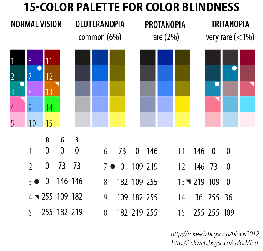
Palettes compatible with colour blindness

Description

Colour palettes recommended for use with colour blind audiences.

Usage

cbPalette8

cbPalette13

cbPalette15

Format

Character vectors of lengths 8, 13 and 15.

An object of class character of length 8.

An object of class character of length 13.

An object of class character of length 15.

Details

Since R 4.0, cbPalette8 is available in base R as palette.colors(8).

cbPalette15 is a Brewer palette. Because colours 4 and 7 are difficult to distinguish from colours 13 and 3, respectively, in individuals with tritanopia, cbPalette13 omits these colours (i.e. cbPalette13 <- cbPalette15[-c(4, 7)]).

Source

cbPalette8: Wong B. 2011. Color blindness. Nat. Methods. 8:441. doi:10.1038/nmeth.1618
cbPalette15: http://mkweb.bcgsc.ca/biovis2012/color-blindness-palette.png

Examples

data("cbPalette8")
plot.new()
plot.window(xlim = c(1, 16), ylim = c(0, 3))
text(1:8 * 2, 3, 1:8, col = cbPalette8)
points(1:8 * 2, rep(2, 8), col = cbPalette8, pch = 15)

data("cbPalette15")
text(1:15, 1, col = cbPalette15)
text(c(4, 7), 1, "[   ]")
points(1:15, rep(0, 15), col = cbPalette15, pch = 15)

Random sample of points for Holdridge plotting

Description

A stratified random sampling (average of 100 points) using a global mapping of Holdridge’s scheme.

Usage

holdridge

Format

An object of class data.frame with 39 rows and 4 columns.

Author(s)

James Lee Tsakalos

Examples

data("holdridge", package = "Ternary")
head(holdridge)

Names of the 38 classes defined with the Holdridge system

Description

holdridgeClasses is a character vector naming, from left to right, top to bottom, the 38 classes defined by the International Institute for Applied Systems Analysis (IIASA).

Usage

holdridgeClasses

holdridgeLifeZones

holdridgeLifeZonesUp

holdridgeClassesUp

Format

An object of class character of length 38.

An object of class character of length 33.

An object of class character of length 38.

Details

holdridgeLifeZones is a character vector naming, from left to right, top to bottom, the 38 cells of the Holdridge classification plot.

holdridgeClassesUp and holdridgeLifeZonesUp replace spaces with new lines, for more legible plotting with HoldridgeHexagons().

Author(s)

Martin R. Smith (martin.smith@durham.ac.uk)

Source

Holdridge (1947), "Determination of world plant formations from simple climatic data", Science 105:367–368. doi:10.1126/science.105.2727.367

Holdridge (1967), Life zone ecology. Tropical Science Center, San José.

Leemans, R. (1990), "Possible change in natural vegetation patterns due to a global warming", International Institute for Applied Systems Analysis Working paper WP-90-08. https://pure.iiasa.ac.at/id/eprint/3443/1/WP-90-008.pdf

The 'Ternary' package allows the creation of ternary plots (a.k.a. ternary graphs / simplex plots / Gibbs triangles / de Finetti diagrams) using the familiar functions of the default 'graphics' package.

Description

Details

Author(s)

See Also

Set plotting region

Description

Usage

Arguments

Value

Author(s)

Examples

Add elements to ternary or Holdridge plot

Description

Usage

Arguments

Functions

Author(s)

See Also

Examples

Annotate points on a ternary plot

Description

Usage

Arguments

Author(s)

See Also

Examples

Colour ternary plot

Description

Usage

Arguments

Value

Author(s)

See Also

Examples

Convert a point in evapotranspiration-precipitation space to an appropriate cross-blended hypsometric colour

Description

Usage

Arguments

Value

Author(s)

References

See Also

Examples

Plot life zones on a Holdridge plot

Description

Usage

Arguments

Details

Author(s)

References

See Also

Examples

Convert user-specified ternary coordinates into X and Y coordinates

Description

Usage

Arguments

Value

Functions

Author(s)

Is a point in the plotting area?

Description

Usage

Arguments

Value

Author(s)

See Also

Examples

Polygon geometry

Description

Usage

Arguments

Value

Functions

Author(s)

See Also

Examples

Reflected equivalents of points outside the ternary plot

Description

Usage