![]()
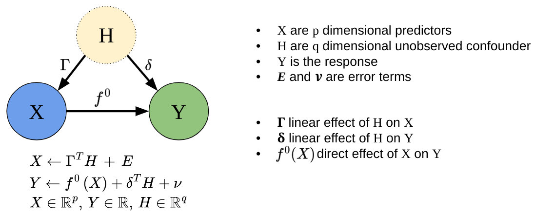
Spectrally Deconfounded Models (SDModels) is a package with methods to screen for and analyze non-linear sparse direct effects in the presence of unobserved confounding using the spectral deconfounding techniques (Ćevid, Bühlmann, and Meinshausen (2020), Guo, Ćevid, and Bühlmann (2022)). These methods have been shown to be a good estimate for the true direct effect if we observe many covariates, e.g., high-dimensional settings, and we have fairly dense confounding. Even if the assumptions are violated, it seems like there is not much to lose, and the SDModels will, in general, estimate a function closer to the true one than classical least squares optimization. SDModels provides software for Spectrally Deconfounded Additive Models (SDAMs) (Scheidegger, Guo, and Bühlmann (2025)) and Spectrally Deconfounded Random Forests (SDForest)(Ulmer, Scheidegger, and Bühlmann (2025)).
To install the SDModels R package from CRAN, just run
install.packages(SDModels)You can install the development version of SDModels from GitHub with:
# install.packages("devtools")
devtools::install_github("markusul/SDModels")
or
# install.packages('pak')
pak::pkg_install('markusul/SDModels')This is a basic example on how to estimate the direct effect of \(X\) on \(Y\) using SDForest. You can learn more about analyzing sparse direct effects estimated by SDForest in the article SDForest.
library(SDModels)

set.seed(42)
# simulation of confounded data
sim_data <- simulate_data_nonlinear(q = 2, p = 50, n = 100, m = 2)
X <- sim_data$X
Y <- sim_data$Y
train_data <- data.frame(X, Y)
# parents
sim_data$j
#> [1] 25 24

fit <- SDForest(Y ~ ., train_data)
fit
#> SDForest result
#>
#> Number of trees:  100
#> Number of covariates:  50
#> OOB loss:  0.1617913
#> OOB spectral loss:  0.05095329
You can also estimate just one Spectrally Deconfounded Regression
Tree using the SDTree function. See also the article SDTree.
Tree <- SDTree(Y ~ ., train_data, cp = 0.01)
#plot(Tree)
Or you can estimate a Spectrally Deconfounded Additive Model, with
theoretical guarantees, using the SDAM function. See also
the article SDAM.
model <- SDAM(Y ~ ., train_data)
model
#> SDAM result
#>
#> Number of covariates:  50
#> Number of active covariates:  3