:warning: Known Issues
The first call of
BayesFluxR_setupcan take a while. On some machines this could take twenty minutes or longer. This is most likely due to that Julia first needs to be set up. If you want to check whether everything is still going well, you can always check in the task manager if the Julia background process is still busy. As long as this is the case, everything is going right.Please always call
library(BayesFluxR)before callingBayesFluxR_setup. CallingBayesFluxR::BayesFluxR_setupthrows an error that I do not know how to solve at this point (feel free to open a pull request)Some systems, especially on company computers, cause failures in the automatic setup of BayesFluxR. In these cases, please try the following
- Install Julia manually by following the official instructions. Link this manual installation to BayesFluxR by calling
BayesFluxR_setup(JULIA_HOME="path-to-julia-binary", env_path="path-to-some-writable-folder", pkg_check=TRUE)or by setting theJULIA_HOMEenvironment variable.- Make sure that the environment path you are choosing is writable. On some systems Julia is not allowed to write to some locations. A safe choice is usually to choose a folder on the Desktop. Note that in the example below I am using the temporary folder on a Mac. This will often not work on company computers.
- If the above still do not work, try to force reinstall BayesFluxR and try the steps again. If it still does not work, please open an issue.
Goals and Introduction
BayesFluxR is a R interface to BayesFlux.jl which itself extends the famous Flux.jl machine learning library in Julia. BayesFlux is meant to make research and testing of Bayesian Neural Networks easy. It is not meant for production, but rather for explorations. Currently only regression problems are being kept in mind during the development, since those are the problems I am working on. Extending things to classification problems should be rather straight forward though, since BayesFlux allows custom implementation of likelihoods and priors (at least in the Julia version). In the R version presented here, this is currently not possible.
BayesFluxR and BayesFlux are based on Flux.jl and thus take over a lot of Flux’s syntax. Before we demonstrate this, we first need to install and load BayesFluxR.
# install.packages("BayesFluxR")BayesFluxR depends on BayesFlux.jl which is a library written in Julia. Hence, to run BayesFluxR, we need a way to access Julia. This is provided by the JuliaCall library. So we also need to install that library.
We are now ready to start exploring BayesFluxR. We first need to load
the package and run the setup. This will install Julia if you do not yet
have it and will install all the Julia dependencies, including
BayesFlux.jl. If you already do have Julia installed, then the script
will pick the Julia version on your computer. If you, like me, have
multiple versions installed, then you can define the version you want to
use by setting the JULIA_HOME variable to the path of the
Julia version you want to use.
Running these lines for the first time can take a while, since it
will possibly have to install Julia and all dependencies. After this, if
you do no longer wish you check if all dependencies are available, you
can set pkg_check = FALSE.
We also set a working environment for Julia. This is generally good
practice and should in real projects be the project directory. It is
also good practice to already set a seed. This seed will be set in both
R and in Julia. If you wish to set a seed later on, please use
.set_seed which sets the seed in both Julia and R.
library(BayesFluxR);
# The line below sets up everything automatically, but sometimes fails
# BayesFluxR_setup(installJulia = TRUE, seed = 6150533, env_path = "/tmp", pkg_check = TRUE)
# If the automatic setup failed or you wish to use a specific version of Julia,
# then use the JULIA_HOME argument. The path below is for a Mac.
BayesFluxR_setup(JULIA_HOME="/Applications/Julia-1.9.app/Contents/Resources/julia/bin/",
             seed = 6150533,
             env_path = "/tmp");
After loading BayesFluxR and running the setup, we are now ready to
experiment around. To create a Bayesian Neural Network, we first need a
Neural Network. In the Flux.jl context and thus also here, a network is
defined as a chain of layers. This is intuitively represented in the
syntax below, which creates a Feedforward Neural Network with one hidden
layer with tanh activation function. The last
Dense(1, 1) statement is the output connection. The chain
below thus says: Feed a vector \(x\)
into the network. Transform this input via \(act=tanh(x'w_1 + b_1)\). The output is
then given by \(\hat{y} = act'w_2 +
b_2\).
net <- Chain(Dense(1, 1, "tanh"), Dense(1, 1))To transform this standard Neural Network into a Bayesian NN, we need a likelihood and priors for all parameters. BayesFluxR view on priors and likelihoods might be a bit unintuitive at the beginning: a prior function only defines priors for the network parameters. Priors for all parameters introduced by the likelihood, such as the standard deviation, are defined in the likelihood functions. So, for example, we can use a Gaussian prior for all network parameters
prior <- prior.gaussian(net, 0.5) # sigma = 0.5and can define a Gaussian likelihood. The Gaussian likelihood also introduces a standard deviation though, which in BayesFlux terms must be given a prior when defining the likelihood: it is not included in the prior above, which applies only to the network parameters. Here we use a Gamma prior for the standard deviation.
like <- likelihood.feedforward_normal(net, Gamma(2.0, 0.5))For all of the estimation methods in BayesFluxR, we need some initial values. BayesFluxR handles this via initialisers, which essentially just tell it how to initialise all parameters. Currently only one kind of initialiser is implemented: Initialising all parameters (network and likelihood) by drawing randomly from a distribution. Users are free to extend this in Julia, but this is currently not feasible in the R version.
# Initialising all values by drawing from a Gaussian
init <- initialise.allsame(Normal(0, 0.5), like, prior)
Now that we have priors on all parameters as well as a likelihood, all that is left is to have some data. Here we will take an AR(1) for the simple reason that time series applications were the first application for which BayesFluxR and BayesFlux were implemented.
n <- 600
y <- arima.sim(list(ar = 0.5), n = 600)
y.train <- y[1:floor(5/6*n)]
y.test <- y[(floor(5/6*n)+1):n]
x.test <- matrix(y.test[1:(length(y.test)-1)], nrow = 1) # In BayesFlux, rows are variables, columns are observations
x.train <- matrix(y.train[1:(length(y.train)-1)], nrow = 1)
y.test <- y.test[2:length(y.test)]
y.train <- y.train[2:length(y.train)]

plot.ts(y, xlab = "", ylab = "", main = "Simulated AR(1) Data")
abline(v = 500, lty = 2, lw = 2, col = "red")
text(x = 500, y = 2.5, labels = "End Training Data", col = "red")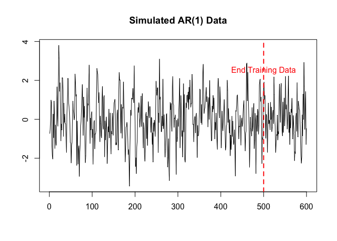
We now have everything to create a Bayesian Model. This is simply
done by calling BNN with the data, the likelihood, the
prior, and the initiliser. The prior and likelihood contain information
about the network structure, and thus it is not necessary to explicitly
give the network structure anymore.
bnn <- BNN(x.train, y.train, like, prior, init)The easiest way to test a BNN and to obtain a first estimate is by
using the MAP or the mode of the posterior distribution. BayesFluxR
achieves this by using stochastic gradient descent type of algorithms.
Currently implemented are opt.ADAM,
opt.RMSProp, and opt.Descent.
# we are using ADAM with a batchsize of 10 and run for 1000 epochs
opt <- opt.ADAM()
mode <- find_mode(bnn, opt, 10, 1000)
We can use this mode estimate to draw from the posterior predictive. Given that the mode is just a single value of the posterior, we will replicate the mode estimate multiple times. This will still only correspond to the one point in the posterior distribution, but will deliver us multiple estimates (multiple draws from the posterior characterised by the MAP).
post_draws <- matrix(rep(mode, 1000), ncol = 1000)
post_values.train <- posterior_predictive(bnn, post_draws, x = x.train)
post_values.test <- posterior_predictive(bnn, post_draws, x = x.test)

yhat.train <- apply(post_values.train, 1, mean)
yhat.test <- apply(post_values.test, 1, mean)
We can now check how good these predictions are:
mse.train <- mean((y.train - yhat.train)^2)
mse.test <- mean((y.test - yhat.test)^2)

c(mse.train, mse.test)
#> [1] 1.045913 1.049174plot(y.test, type = "l", xlab = "Time", ylab = "", main = "Test data performance", col = 1)
lines(yhat.test, col = 2)
legend(x = 0, y = 3, c("y", "yhat"), col = c(1, 2), lty = c(1, 1))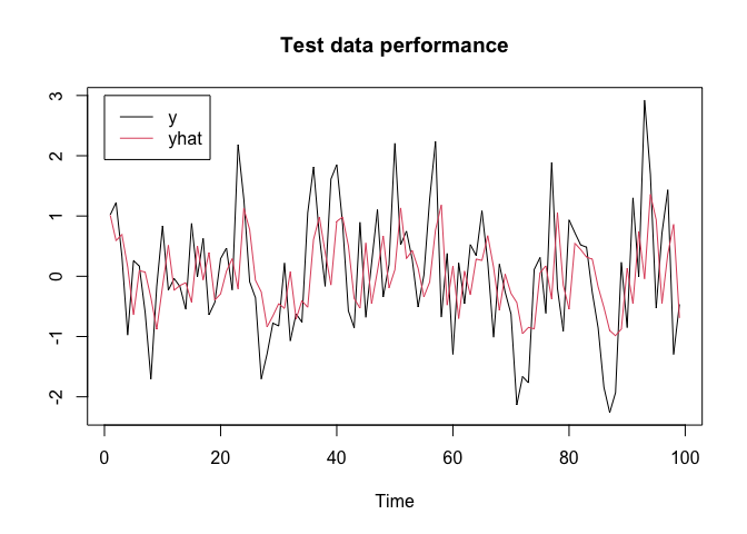
The next step up from a MAP estimate is a Variational Inference estimate. BayesFluxR currently implements Bayes by Backprop (BBB) (Blundell et al. 2015) using a Multivariate Gaussian with diagonal covariance matrix as proposal family. Although BBB is the standard in Bayesian NN, it can at time be restrictive. For that reason, BayesFlux allows for extensions in the Julia version, not currently though in the R version.
# using a batchsize of 10 and running for 1000 epochs
vi <- bayes_by_backprop(bnn, 10, 1000)
BBB does not itself return posterior draws yet. Instead, it returns information about how the distribution looks like, restricted by it being a Multivariate Gaussian with diagonal variance. To actually obtain draws, we still need to sample from this variational family.
post_samples <- vi.get_samples(vi, n = 1000)We can then use these draws like we would use any other posterior draws. For BNNs we are usually not interested in the actual parameters, but rather in the posterior predictive distribution. As such, we can use these draws to obtain posterior predictive draws.
post_values.train <- posterior_predictive(bnn, post_samples, x = x.train)
post_values.test <- posterior_predictive(bnn, post_samples, x = x.test)

yhat.train <- apply(post_values.train, 1, mean)
upper.train <- apply(post_values.train, 1, function(x) quantile(x, 0.975))
lower.train <- apply(post_values.train, 1, function(x) quantile(x, 0.025))

yhat.test <- apply(post_values.test, 1, mean)
upper.test <- apply(post_values.test, 1, function(x) quantile(x, 0.975))
lower.test <- apply(post_values.test, 1, function(x) quantile(x, 0.025))


data.frame(
  mse.train = mean((y.train - yhat.train)^2),
  mse.test = mean((y.test - yhat.test)^2),
  coverage.train = mean(((y.train < upper.train) & (y.train > lower.train))),
  coverage.test = mean(((y.test < upper.test) & (y.test > lower.test)))
)
#>   mse.train mse.test coverage.train coverage.test
#> 1 1.051824 1.038127 0.9418838 0.9494949BayesFluxR implements various Markov Chain Monte Carlo methods that can be use to obtain approximate draws from the posterior. Currently implemented are
sampler.SGLDsampler.SGNHTSsampler.GGMCsampler.HMCsampler.AdaptiveMHAdditionally, BayesFluxR allows for adaptation of mass matrices and stepsizes for some of the samplers above:
madapter.DiagCov,
madapter.FullCov, madapter.FixedMassMatrix or
madapter.RMSProp can be done for SGNHTS, GGMC, and HMCsadapter.Const or
sadapter.DualAverage can be done for GGMC and HMC since
these two are the only samplers using both gradients and a
Metropolis-Hastings accept/reject step.# sampling via sgld
sampler <- sampler.SGLD(stepsize_a = 1.0)
samples.sgld <- mcmc(bnn, 10, 10000, sampler) # batchsize 10 and 1000 samples
# sampling via SGNHTS
sampler <- sampler.SGNHTS(1e-2)
samples.sgnhts <- mcmc(bnn, 10, 10000, sampler)
# sampling using GGMC with fixed mass but stepsize adaptation
madapter = madapter.FixedMassMatrix()
sadapter = sadapter.DualAverage(1000, initial_stepsize = 1) # 1000 adaptation steps
sampler <- sampler.GGMC(l = 1, sadapter = sadapter, madapter = madapter)
samples.ggmc <- mcmc(bnn, 10, 10000, sampler)
# sampling using HMC
# This time batchsize is is length of y thus no batching
sadapter <- sadapter.DualAverage(1000, initial_stepsize = 0.001)
madapter <- madapter.FixedMassMatrix()
sampler <- sampler.HMC(l = 0.001, path_len = 5, sadapter = sadapter, madapter = madapter)
samples.hmc <- mcmc(bnn, length(y.train), 10000, sampler)
# sampling using Adaptive MH
# this does not use any gradients so we start at a mode
sampler <- sampler.AdaptiveMH(bnn, 1000, 0.1)
samples.amh <- mcmc(bnn, 10, 10000, sampler, start_value = mode)All of these samples can be used in the same way. For example, we can use the samples obtained using SGNHTS to draw from the posterior predictive. We are again not really interested in the actual parameters, but much more in the posterior predictive values and the network output space.
post_values.train <- posterior_predictive(bnn, samples.sgnhts$samples, x = x.train)
post_values.test <- posterior_predictive(bnn, samples.sgnhts$samples, x = x.test)


yhat.train <- apply(post_values.train, 1, mean)
upper.train <- apply(post_values.train, 1, function(x) quantile(x, 0.975))
lower.train <- apply(post_values.train, 1, function(x) quantile(x, 0.025))

yhat.test <- apply(post_values.test, 1, mean)
upper.test <- apply(post_values.test, 1, function(x) quantile(x, 0.975))
lower.test <- apply(post_values.test, 1, function(x) quantile(x, 0.025))


data.frame(
  mse.train = mean((y.train - yhat.train)^2),
  mse.test = mean((y.test - yhat.test)^2),
  coverage.train = mean(((y.train < upper.train) & (y.train > lower.train))),
  coverage.test = mean(((y.test < upper.test) & (y.test > lower.test)))
)
#>   mse.train mse.test coverage.train coverage.test
#> 1   1.04987 1.048984      0.9438878     0.9494949
It is often a good idea to check whether at least the parameters additionally introduces by the likelihood have reasonable chains. Although better statistics exist, here we will only check it visually. Sigma is here given by the last parameter. In general, if the likelihood introduces k parameters, then the last k parameters in each draw are those of the likelihood.
s <- samples.sgnhts$samples
sigma <- s[nrow(s), ]
plot.ts(sigma)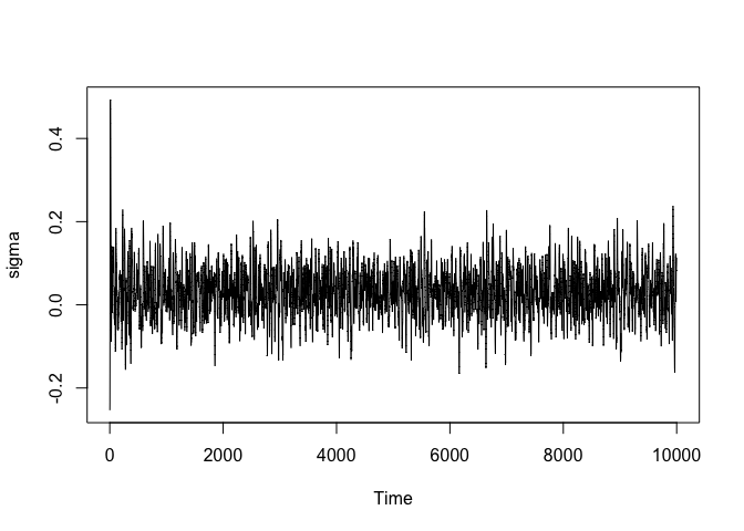
What if we were not happy or if the chain had not yet converged? In that case we can just continue sampling instead of having to start fresh.
samples.sgnhts.cont <- mcmc(bnn, 10, 20000, sampler = samples.sgnhts$sampler, continue_sampling = TRUE)

list(
  dim(samples.sgnhts.cont$samples),
  all.equal(samples.sgnhts$samples, samples.sgnhts.cont$samples[, 1:10000])
)
#> [[1]]
#> [1]     5 20000
#>
#> [[2]]
#> [1] TRUENext to Dense layers, BayesFluxR currently supports the use of RNN and LSTM layers. Currently only seq-to-one tasks are supported (only those likelihoods are implemented) and extension possibilities do currently only exist in the Julia version, but the plan is to update this soon.
Say we have a time series \(y\) with possibly non-linear dynamics. We can then split this time series into overlapping subsequences and use each of these subsequences to predict the value that would come in \(y\) after the subsequence ends. This way we can train an RNN or LSTM network with a single time series.
To support the above, BayesFluxR comes with a utility function
tensor_embed_mat which takes a matrix of time series and
embeds it into a tensor consisting of dimensions \(seqlen \times numvariables \times
numsubsequences\).
# We want to split the single TS into overlapping subsequences of
# length 10 and use these to predict the next observation
y <- arima.sim(list(ar = 0.8), n = 600)
tensor <- tensor_embed_mat(matrix(y, ncol = 1), len_seq = 10 + 1)
dim(tensor)
#> [1]  11   1 590
We now have a tensor with subsequences of length 11, the first 10 elements of each sequence are used to predict the 11th element.
y.rnn <- tensor[11, , ]
x.rnn <- tensor[1:10, , ,drop = FALSE]

train_to <- floor(5/6 * length(y.rnn))
y.train <- y.rnn[1:train_to]
y.test <- y.rnn[(train_to+1):length(y.rnn)]
x.train <- x.rnn[, , 1:train_to, drop = FALSE]
x.test <- x.rnn[, , (train_to+1):length(y.rnn), drop = FALSE]
After bringing the data into the right format above, the rest of the functionality is the same as for Feedforward architectures:
net <- Chain(RNN(1, 1), Dense(1, 1))
prior <- prior.mixturescale(net, 2.0, 0.1, 0.99)
like <- likelihood.seqtoone_normal(net, Gamma(2.0, 0.5))
init <- initialise.allsame(Normal(0, 0.5), like, prior)
bnn <- BNN(x.train, y.train, like, prior, init)
One thing not discussed above is that BayesFluxR also allows to draw from the prior_predictive distribution. This often shows that the priors currently used in standard work are often not the best and much work could be done here.
prior_values <- prior_predictive(bnn, n = 10)
plot(x = 1:length(y.train), y = y.train, type = "l", xlab = "Time", ylab = "", main = "Prior Draws", col = "red")
for (i in 1:ncol(prior_values)){
  lines(prior_values[, i], col = "black", lty = 2)
}
legend("topright", c("Training Data", "Prior Draw"), col = c("red", "black"), lty = c(1, 2))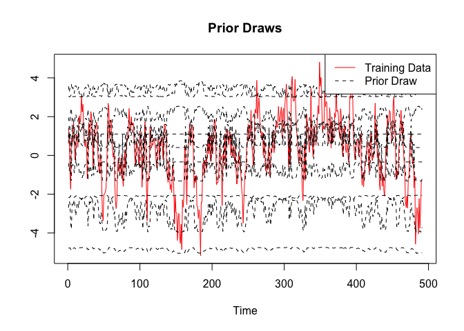
Estimation works the same as for Feedforward structures. For example, we can estimate the model using SGNHTS
sampler <- sampler.SGNHTS(0.01)
chain.mcmc <- mcmc(bnn, 10, 10000, sampler)
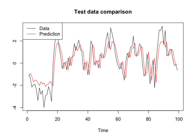
And obtain the posterior predictive draws for the test data and compare it to the actual values:
post_values.test <- posterior_predictive(bnn, chain.mcmc$samples, x = x.test)

yhat.test <- apply(post_values.test, 1, mean)
plot(y.test, type = "l", xlab = "Time", ylab = "", main = "Test data comparison", col = "black")
lines(yhat.test, col = "red")
legend("topleft", c("Data", "Prediction"), col = c("black", "red"), lty = c(1, 1))